Reception of (strange) VLF – signals
with a PC
from
Harald Lutz
Nowadays
the most convenient and
simplest way to receive VLF – signals is using a PC. If a
PC with soundcard is
already available, it is also the cheapest method. You
need only a coil (as coil
you can use a roll of insulated wire, the electrical data
of the coil are very
uncritical), a cable with a length of at least 1metre and
a plug for connecting
the cable to the input of the soundcard (the necessary
software is as free- or
shareware available in the internet). Together this device
costs you only
approximately 10 Euro!
Since
cables with soldered plug for all
kind of soundcard entrance sockets can be bought readily
you only have to
solder the coil to the free end of the cable in order to
get a VLF – aerial for
your PC! Another advantage of VLF – reception with a
PC is, that you can
in opposite to a conventional receiver examine multiple
signals simultaneously.
In
principle it is possible to analyse
all signals in the frequency range between 0 Hz to 22.05
kHz ( respectively 24
kHz) at the same time with your device! Further you
can record all
received signals -either as wav – file-or as spectrogram
in form a bitmap or
jpeg.
This
process can be easily automated, so
you need not to be at your computer and wait for
interesting signals!
But
using a PC as VLF – receiver has two
disadvantages: first you cannot receive
(with the customary device) signals with frequencies above 22.05 kHz
(respectively 24 kHz when your
hard- and software allows sampling with 48 kHz), second
and this is more
important, the computer and its peripherical device are
sources of disturbing
signals.
Especially
the monitor of a PC is a
powerful source of interference in the VLF – range!
My Equipment
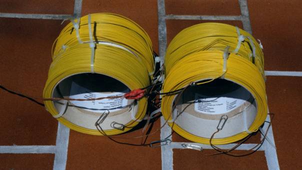
A) Aerial
As aerial I use an
inductive aerial, which consists
(at the moment) of a serial connection of 2 coil units.
Each of these coil units consists of
2 identical part coils.
These part coils are rolls of
insulated copper flex and can be bought ready – made in an
electronic store, so
there is no work necessary to coil them.
Originally they are designed as a
storage for copper flex and not for a usage as inductivity or
electromagnet.
|
|
|
Photograph of my VLF – aerial Technical data:
|
The coil units are laid in that way
on the floor of my room or of my balcony, that their axis show
in the desired
direction ( e.g. north – south or east – west).
This orientation of the axis of the
coil units is very important, because it shows as all
inductive aerials a
strong directional effect. (In the description of my
spectrograms you will
always find a giving in which direction the axis of the coils
showed).
My aerial system grew with the time.
At the beginning I used only one wire roll, then two and at
the moment I use
four.
In normal operation a serial
connection of all four part coils is used, but I can for test
purposes short –
circuit each
part coil
individually by the help of paperclips, which are connected to
the connection
of each part coil.
The aerial is directly
-without using a
preamplifier- connected
with a 2
metre long unshielded twisted – pair
cable with the line – input of my PC.
B)
Hardware and modes of operation
My PC has a Pentium –
III MMX processor with a beat
frequency of 500 MHz.
It uses a Windows98 operating
system.
Its soundcard is a Sound Blaster Audio
PCI128. Although this soundcard can sample signals with a
frequency of 48 kHz,
most analysis were performed until August 23rd, 2001 with 44.1
kHz, because
analysis software for a sampling rate of 48 kHz was barely
available until this
day.
( Since August 23rd, 2001 the
spectrum analysis software SpecPlus is available in a new
version, which allows
the employment of a sampling rate of 48 kHz.)
At my reception site not much space
is available.
My monitor is only approximately 3
metres away from my aerial, so the noise from my monitor
disturbs the VLF
reception considerably. In order to avoid these disturbations,
I use
"offline – reception", that means
I make screenshots of the
spectrograms with the monitor turned off and save these
screenshots as graphic
file.
Therefore I use manually the
"Print Screen" key or let this job do periodically by a
special
software.
Of course I have no direct visible
control of my spectrograms that I capture, but by automatic
recording, I can
record all signals when I sleep or when I am not at home.
And at late night the disturbation
level is lowest!
C)
Software
5 programmes are in use
at my PC in the moment:
Spectrogram Version 5.1.7, Spectrogram Version 6.2, Spektran
beta 4, build
127, Spektran
Version 1.0 and
SpecPlus.
Each of these programs has their
advantages and disadvantage.
Spectrogram Version 5.1.7 I use only
to get a quick overview of the actual situation in the VLF –
range. I do not
make any recordings with it any more.
Spectrogram 6.2. allows sampling with
48 kHz, but I think the way how Spektran shows the results is
much nicer, so I
use Spektran more likely then Spectrogram, although Spektran
often leads to
system crashes and Spektran 1.0, which allows also the usage
of a sampling rate
of 48 kHz, does not allow the simultaneous examination of a
frequency range of
more then 5.7 kHz of the VLF – range.
For automatic recording in
combination with all versions of Spectrogram and Spektran I
use 2020, Version
2.2.7, but unfortunately after at the latest 125th
screenshot the programme stops its operation (when you do not
have enough space
on your hard disk then it stops earlier!), so I use for
automatic long time
reception, SpecPlus.
This software allows in its actual
version, which is since August 23rd, 2001 available, the usage
of a sampling
rate of 48 kHz and saving spectrograms in constant intervals
as bitmap or jpeg
– file.
SpecPlus does not make -even after
long time operations- the system crash.
It can record data as long as your
drive, on which the data are saved, is full.
But 2020 is not obsolete when using
SpecPlus. This programme can be used in order to convert
recorded bitmaps – in
jpg – files or to transform the recorded jpgs in jpgs of
smaller file size.
If you want to download one of the
upper mentioned software, then look on the following table:
Since version changes
very often, the upper mentioned
versions can be not available any more.
|
Software |
Internet
page
|
|
Spectrogram Spektran SpecPlus |
Observations
Fields of interest
My
major field of interest in reception of signals below 24 kHz
are the man – made
signals.
I am
interested in their strength, form, direction and the time
when they occur.
From
these signals my major attention is on the signals of the
transmitters.
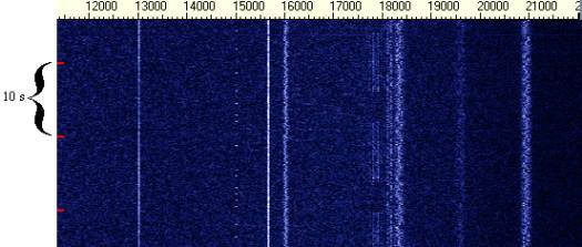
Regular signals:
- Transmitters
usually you will find at
least the signal of one of
the following transmitters on your recording
|
Call sign |
Frequency |
Location |
|
GBR JXN RDL/UPD/UFQE/UPP/UPD8 HWU GBZ ICV HWU HWU |
16.0 kHz 16.4 kHz 18.1 kHz 18.3 kHz 19.6 kHz 20.76 kHz 20.9 kHz 21.75 kHz |
Rugby (UK) Helgeland
(Norway) Russia
(different locations) Le Blanc
(France) Criggion (UK) Tavolara (Italy) Le Blanc
(France) |
None of these transmitters is
permanently on the air. So you do not wonder if you cannot
receive one of the
listed stations. Do not expect ever to receive all these
stations
simultaneously.
If your hard- and software allows a
sampling rate of 24 kHz, you can also receive the signal of
DHO38 on 23.4 kHz,
the transmitter of the German Navy located near West –
Rhauderfehn, North
Germany (Coordinates: 53N05 7E40).
Further you can find sometimes on
spectrograms showing the range between 22 kHz and 24 kHz a
weak signal just
below 24 kHz. It comes either from NAA in Cutler (USA), NSS in
Annapolis (USA),
NBA in Balboa (Panama), NLK in Oso Wash (USA) or NPM in Pearl
Harbour (Hawaii).
|
|
|
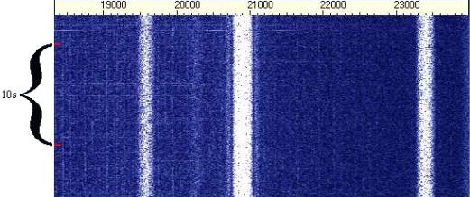
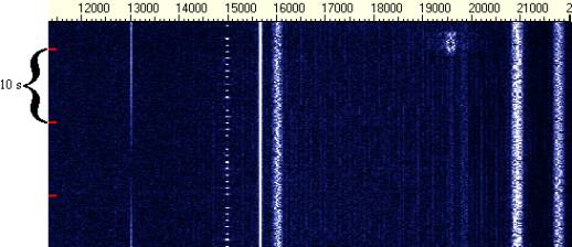
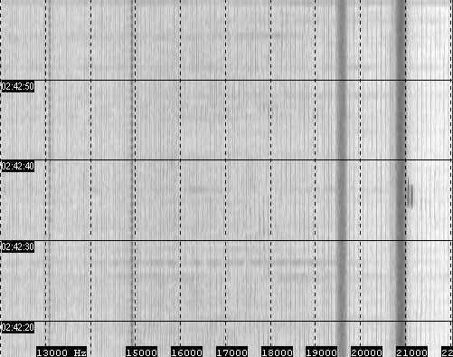
August 10th, 2001 at
13h56m44s UT Frequency range between 18.3 kHz and
24 kHz The axis of
the reception coils showed in North – South –
direction, Analysis software: Spektran
Version 1.0 You will
find on it the signal of GBZ on 19.6 kHz, of ICV
on 20.27 kHz, of HWU on 20.9 kHz, of DHO38 on 23.4
kHz. Further you will find just below 24 kHz a
weak signal which comes presumably from NAA or
NSS, since these transmitters are from all
transmitters working on 24 kHz closest to my
reception side. |
A
more detailed list of VLF – transmitters you will find on http://www.vlf.it/itulist/itulist.htm.
- Signals from
electrical device
Several signals from
electrical device occur in the
VLF – range. The most important one is the TV line scan base
frequency on
15.625 kHz. This signal can be detected in a radius of several
metres around
every running TV – set.
Other sources of VLF – emission are
switching transformers and neon tubes.
Their frequencies are very different
and depend on the type and model of
device.
This is also valid for the VLF –
signals of PCs. Concerning PCs another problem occurs, since a
computer does
not always emit the same signals in the same intensity.
They can sometimes change their
strength in a very uncharacteristic pattern.
Because of this fact it is not
always easy to find out, if a signal comes from your computer
or not.
In order to do this job, it is best
for comparison to analyse the VLF – range with a second
computer at the same
time.
Of course both computers should use
the same software with the same settings and examine the same
frequency range.
Further attention must paid to, that
the orientation of the reception coils of both computers is
the same and that
the aerial is more then 2 metres away from the comparison
device (including its
aerial).
Otherwise its signals would be
received.
If a second computer is not
available, disconnect or short – circuit the reception coil.
Signals from
external sources must then disappear!
(In my following
spectrograms two noise signals from
my PC are existing. One on 13 kHz and an other on 15 kHz)
Irregular signals
The
most interesting signals in the VLF – range are the irregular
signals. They can
have their origin in a known or unknown source.
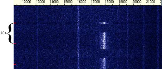
- Funny signal of Criggion
VLF
– transmitter generate, when they test their modulator,
sometimes funny
signals, which look like garlands or fishes. So did the
transmitter Criggion at
the end of June 2001.
|
|
|
June 21st, 2001 16h37m43s UT:
Garlands from Criggion
|
|
|
|
June 21st, 2001 18h25m14s UT: A long garland from Criggion
|
|
|
|
June 22nd, 2001 18h39m44s UT: A signal from Criggion that looks
like a fish
|
-Time - signal
stations of the former Soviet – Union
There are several time – signal
stations in the former Soviet – Union which works in the VLF –
range.
These stations are RJH63 in
Krasnodar (Russia), RJH66 in Bishkek (Kyrgyztan), RJH69 in
Moldechno (Belarus),
RJH77 in Arkhangelsk (Russia), RJH99 in Nizhny Novgorod
(Russia) and RAB99 in
Khabarowsk (Russia).
These transmitters are not
permanently on the air, but transmit alternately according to
a complicate
scheme on the frequencies 20.5 kHz, 23 kHz, 25 kHz, 25.1 kHz
and 25.5 kHz.
(Further information can be found on
http://www.vlf.it/russianvlf/russianvlf.htm)
With a PC – soundcard you can only
receive the signals on the frequencies 20.5 kHz and 23 kHz.
For the reception of the signals on
25 kHz, 25.1 kHz and 25.5 kHz a special VLF – receiver is
required.
-Signals from RJH66,
RJH69, RJH77, RJH99 and RAB99
If for the reception only the
soundcard of the PC is available, these transmitters are
unfortunately not easy
to identify, because they emit on the frequencies 20.5 kHz and
23 kHz only an
unmodulated carrier.
Such a signal can be easily confused
with a jam signal, e.g. from a switching transformer.
The best criterion to identify
signals from RJH66, RJH69,
RJH77, RJH99 and
RAB99, is to search on the spectrograms for the end of the
transmission.
The transmission on the frequency
20.5 kHz is terminated 17 respectively 47 minutes after the
begin of the full
hour.
|
|
|
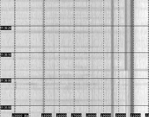
October 3rd, 2001: RJH77 terminated its transmission on 20.5kHz The
reception coil was oriented in East – West –
direction. The time value is in Middle European
Standard Time. Recording software was SpecPlus. The scroll – interval was 0.01s,
frequency resolution: 0.6729 Hz |
On the frequency 23 kHz the end of
the transmission takes place 11 respectively 41 minutes after
the beginning of
the full hour.
|
|
|
October 3rd, 2001: RJH77 terminated
its transmission on 23kHz The
reception coil was oriented in East – West –
direction. The time value is in Middle European
Standard Time. Recording software was SpecPlus. The scroll – interval was 0.01s,
frequency resolution: 0.6729 Hz |
On both frequencies the end of transmission occurs very
suddenly.
The beginning of the transmission of
these signals takes place for the frequency 23kHz 5
respectively 35 minutes and
for the frequency 20.5 kHz 11 respectively 41 minutes after
the begin of the
full hour.
It is only weak distinct on the
spectrograms, because the intensity of the transmitted carrier
grows slowly and
continuously.
Because of that it can be not always
detected, if local sources of disturbance are present.
-Signals
of RJH63
The
signal of RJH63 is
somewhat easier to identify.
This transmitter emits the days, on which it is running, between 11h 36m UTC * and the end of the transmission at 11h 40m UTC* a frequency modulated signal with a shift of 300 Hertz.
|
|
|
August 5th, 2001: A signal of RJH63 The
reception coil was oriented in North – South –
direction. The time value is in Middle European
Standard Time. Recording software was SpecPlus. The scroll – interval was 0.01s,
frequency resolution: 0.6729 Hz |
Unfortunately
the signal
of RJH63 on the frequency 23 kHz is also unmodulated.
It
can be best
identified by its sudden end at 11h 31m UTC*.
Like
the others VLF time
– signal transmitters of the former Soviet Union, the
beginning of the
transmission on 20.5 kHz and 23 kHz is also only weak distinct
for RJH63, too,
because the strength of the signals at the begin of
transmission (11h 26m UTC*
for 23 kHz and 11h 31m UTC* for 20.5 kHz) grows only slowly.
* 1 hour later during
summer time
-Rarely
active transmitters
Some VLF – transmitters mentioned in
the tables as http://www.vlf.it/itulist/itulist.htm.are
only
very rarely on the air.
One of these transmitters is RDL
(Russia) on 21.1 kHz, which transmitted on August 5th, 2001
only for a few
seconds! (See below)
|
|
|
August 5th, 2001: A signal of RDL The
reception coil was oriented in North – South –
direction. The time value is in Middle European
Standard Time. Recording software was SpecPlus. The scroll – interval was 0.01s,
frequency resolution: 0.6729 Hz |
Two further well – receiveable VLF –
stations which are only exceptionally in service are UMB
(located near Rostov,
Russia) on 18.9 kHz and ICV (Location: Tavolara, Italy) on
20.27 kHz..
(The standard frequency of ICV is
20.76 kHz where it can be received very often).
But do not forget, in this chapter
the situation of summer 2001 is described.
Short term – changes in
transmitting activity are
always possible, so a transmitter which is at the moment very
rarely on the air
can be very active at a later point of time!
- Signals on 17.8 kHz
Sometimes
I detected signals on 17.8 kHz. Apparently a transmitter is
tested on this
frequency, since I could not receive regular signals on this
frequency.
|
|
|
May 24th, 2001 13h03m28s UT: A signal
on 17.8 kHz
|
|
|
|
June 23rd, 2001 16h07m45s UT: A signal on 17.8 kHz
|
According
to ITU lists the frequency 17.8 kHz is allocated to
transmitters in different
locations in the USA and the frequency 17.9 kHz to a
transmitter in the eastern
part of Russia. But, if the recorded signal comes from one of
these
transmitters, why is it much stronger then the signals of GBR,
GBZ and HWU?
- An unidentified transmitter on 15.8
kHz
|
|
|
July 12th, 2001 15h12m45s UT: Reception of a signal on 15.8 kHz
|
What is
its origin?
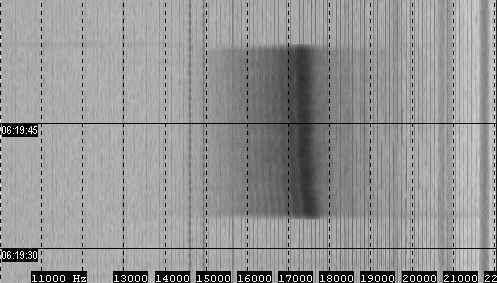
- Short pulses in the range between 17
and 18 kHz
Sometimes in the range
between 17 and 18 kHz short
pulses with a duration of approximately 20 seconds occur. They
have a big
bandwidth and sometimes an enormous intensity.
|
|
|
Strong pulse between 17 and 18 kHz
recorded on the morning of July 27th, 2001
|
|
|
|
A similar, but weak pulse recorded a
day later. The time value is in Middle European
Standard Time
|
Occurrence
During an automatic session on
August 5th, 2001 these pulses were registered at following
times:
(all time values in UT)
|
Strong pulse |
Weak pulse |
|
4h 08m
50s 5h 53m |
3h 03m 4h 07m
45s 6h 43m
30s 7h
25m 20s 11h
39m |
All these pulses look like the
pulses shown in the spectrograms above.
Because weak pulses are more frequently
then strong pulses, I suppose that both types originate in the
same way and
come from sources, which are in different distances of the
reception side.
The question is: what are these
sources?