The following is an analysis of a number of samples taken from the various audio files gathered during the field investigations carried out in Hessdalen in August 2000 [1] in order to study any correlation between VLF emissions and the well-known light phenomenon. The recordings were made with a VLF receiver known as ELFO (Extremely Low Frequency Observatory [2]) created at the CNR Institute of Radio Astronomy. The correlation receiver operates from 100Hz up to 22KHz and exploits two 2x2m loop antennas.
The files analysed represent a selection of signals considered abnormal when compared to the spectrum of electromagnetic emissions which may be expected. The analysis was performed using SpectrumLab V 2.5 b1,with various resolutions in time and frequency aimed at identifying the nature of the emissions. The spectrograms shown in this article were all carried out with a 1024-dot FFT and a scroll time of 15 ms.
SIGNAL ANALYSIS
The spectrograms below show the FFT analysis across the bandwidth. The various technical data included in the comments refer to analyses carried out on the same file using high frequency resolution in order to highlight some of the aspects linked to the spacing of the signal frequencies, and in some cases with a few FFT dots so as to determine exactly their evolution over time.
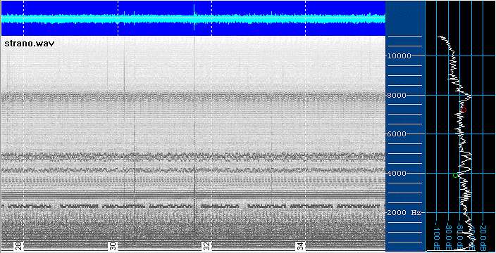
SAMPLE n.1
The background network hum is very pronounced, due
to the number of inverters found along the valley and electronic power
commutation, and is not of a particularly stable frequency (something which
becomes clear by raising the number of FFT analysis points). We should
point out that in Hessdalen (as in the whole of Norway) there are no pipelines
for the transport of gas. Thus Norwegians rely exclusively on the supply
of electricity for all their domestic requirements. Clearly, much of this
equipment requires electronic power commutation or straightening. The 50
Hz harmonics are dominant here, typical of the straightening of an insufficiently
filtered sinusoidal signal. The rising and falling noise is often due to
some sort of regulation, and is often found near power lines, as may be
seen in the spectrogram. This type of signal has a particularly strong
magnetic component due to the passage of electric current through the network
conductors. The signal found at 2300 Hz is the beat of a time station sample
(MSF or DCF) with an RTTY spaced out over the 2300 Hz frequency: the front-end
of the receiver is intermodulating. This phenomenon is clearly visible
thanks to the cadence of the tones, exactly one second apart. When the
Omega stations were still working, the problem was in fact much greater.
It was common to see spectrograms (especially if taken from a certain altitude)
with Alpha and Omega emissions transferred within a few kHz of each otherÕs
beats. For this reason, if one overdoes the gain level, there is a risk
of calibrating the front-end of a receiver where no intermodulation phenomena
are present only to find it to be faulty when transported elsewhere.
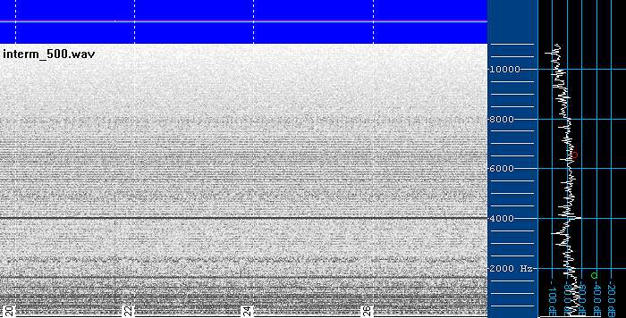
SAMPLE n.2
This is a "low hum" of artificial nature, clearly
to do with the electric supply, for the bands of cyclical vertical noise,
shown in detail, turn out to be comb of harmonics each exactly 100 Hz apart.
This signal may be picked up with a certain regularity in zones of industrial
activity. Given how it uses electricity network conductors as a means of
propagation, the signal may be picked up several miles away from its original
source. It usually has a very strong magnetic component and a strong electrical
component on a ground level yet weak if picked up using floating electrical
systems. The same goes for the bands of noise below 1 kHz, commonly found
within 15km of power lines.
The band of noise found around 8 kHz is usually
provoked by the triac regulation of the power supply for street-lighting
systems.
SAMPLE n.3
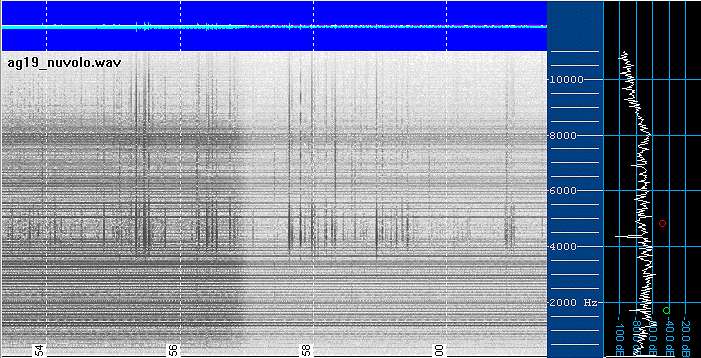
The same "network hum", which at a certain point
disappears, making the band visible once again. The same signals can be
seen with the auxiliary of a single-coil network transformer accessing
the sound card directly: the distribution takes place via the electric
network. When this interference disappears, the even network harmonics
can be seen once more to provide a constant background noise, along with
a few instances of storm-cloud static discharge, albeit very weak when
compared to the intensity of the electrical disturbances.
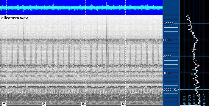
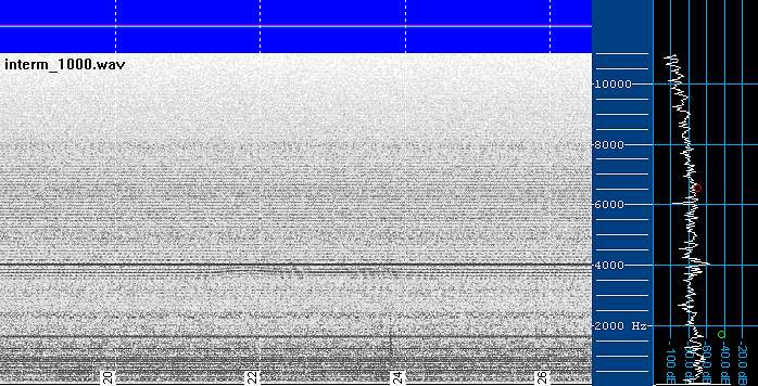
SAMPLE n.4
A recording made some time later. The intensity
of the RTTY signals is greater due to the propagation and the front-end
of the receiver, which earlier on was giving signs of intermodulation and
which now acts like an RF mixer, returning the differences between signals
in the HF band to the base band. The band below 6 kHz thus appears full
of non-existent signals and images due to the non-linearity of the first
amplification stage. Here we may also find the usual network harmonics
together with the signal of an electric motor passed through the distribution
network. The sound is similar to that of a dentist's drill, and a close
look at the spectrogram shows that it is made up of a comb of harmonics
exactly 100 Hz apart. This type of signal, which exploits the distribution
network, may spread for a number of miles from its original source.
SAMPLE n.5
Network harmonics, the beat between STC and RTTY
at 2250 Hz, a continuous tone at 4 kHz and some very faint remote static
interference below 1 kHz. What emerges in particular from this is that
the disposition of the network harmonics constitutes a homogeneous background
up to and beyond 8 kHz. This leads us to imagine that the origin of the
disturbance is not far away. In fact, the fading of the section increases
along with the increase in frequency at the same distance

Generally speaking, it is rare to be able to pick
out a harmonic comb of 50 Hz at frequencies above 9 kHz especially in particularly
noisy, disturbed environments in which the source of the disturbance is
relatively far away.
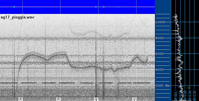
SAMPLE n.6
A weak beat present at 2250 Hz. The harmonic curve
(seen around second 22) shows the presence of a disturbance originating
from an electricity-generating unit unable to maintain a constant rotation
speed, or one in which the alternating current generated by an inverter
has a somewhat unstable frequency. There is some faint, remote static interference
under 2 kHz after second 24 but of very low intensity. This makes it hard
to define the true source of the noise (in the spectrum on the side with
an average value around an arbitrary -80 dB) and thus whether it is of
natural origin or whether it is a man-made or microphonic disturbance due
to the mechanical movement of the antenna.
By way of example, the following is a spectrogram carried out in Cumiana (province of Turin, Italy) which shows what might usually be found in the monitoring of audio bands.

The parameters of the FFT analysis are the same as those of the Hessdalen spectrograms. Static discharges of natural origin may be seen, and under 2 kHz, there are network harmonics (for the reception was carried out in a back garden. The sharp static curves around 2 kHz (second 24) are an effect of propagation and are known as tweeks.
INTERMODULATION PHENOMENA
These are altogether less surprising than one might at first imagine, especially for those of us who are in a certain sense more used to dealing with VLF and ELF bands. The development of an audio band receiver, while circuit-wise very simple, actually requires a great amount of time for the fine tuning that follows. This is because it is really quite difficult in a laboratory to recreate the conditions later found in the field. Furthermore, field conditions may alter greatly and change even after long periods of time. Thus, it can happen that a receiver developed and tested for a number of months may suddenly start to give problems due to the presence of signals at frequencies higher than those contemplated and of great intensity.
To get an idea of what this means, think of a far simpler circuit such as that of the EasyLoop (a single-operational receiver and a loop of 40 coils only 75cm in diameter [3]) which was developed in the lab in just three days, but of which the debugging stage required a further two months before the most part of the intermodulation phenomena had been eliminated.
With this end in mind, a number of filters were added to the circuit; something which might appear bereft of sense in electric terms, but which once inserted, made it possible for the operational to work in a linear fashion. The explanation is simple: the theoretical behaviour of the operational is valid only up to a certain frequency limit, as conditioned by the chosen factor of amplification.
It may be that the amplification systems used by
ELFO suffer from the fact that in the presence of strong signals (far higher
than those received under test conditions at the INAF on the radio telescopes
of Medicina), the intermodulation phenomenon generates superfluous signals
which are not in fact present in the reception band.
THE ORTHOGONAL LOOPS
Previous experiments carried out in order to identify the presence of very faint signals embedded in noise have shown that a technique supplying better results may be found via the use of two receivers in an orthogonal set-up. The two loops already created could be positioned in the same place but at right angles and the two signals used to elaborate a complex FFT. The spectrogram illustrates an example of this technique as applied to the 0 to 103 Hz range for the study of radio-seismic precursors.
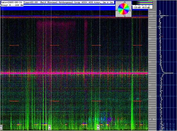
In this image, various types of signal may be made
out coming from different directions: from the 50 and 100 Hz network signals
to the mirrored signals around 50 Hz, Schumann resonance, storm-cloud static
within the range of a few hundred kilometres, natural geomagnetic pulsation,
as well as microphone effects due to small loop vibrations. From a single
spectrogram of this type, a truly vast amount of information may be gathered.
The colour of the signals denotes the phase with which they are received; thus in the case of a remote field, also the incoming direction of the signals. The colour saturation level, on the other hand, indicates the intensity of the signal itself. This technique, apart from revealing signals which are at any rate visible on a normal spectrogram, also allows for the visualisation of imperceptible variations in the background noise based solely on its phase variations. For example, it is fairly common to see the colour of the background noise change for a certain time while a common spectrogram or signal intensity plot of the same frequency range may show up nothing at all. Furthermore, this technique allows for the software suppression of a particular direction of incoming signal, thus eliminating network hum from the spectrogram before it even gets that far.
CONCLUSION
Given the absence of anomalous signals compared with what may be recorded in any area of the countryside, it would be good if in the following field trips we were lucky enough to have an optical recording backup, which would at least make it possible to draw a link between the optical phenomenon and any VLF radio ones.
The spectrograms do not indicate any anomalous phenomenon: all the signals analysed are commonly receivable while listening to Radio Nature in country areas not too far away from urban areas. If the monitoring is carried out with loop receivers (such as ELFO), disturbances may be sensed due to its sensitivity even a number of miles from the origin of the source. The electric network, thanks to its all-engulfing distribution pattern, creates a series of rings in which the magnetic signal is induced like in gigantic spirals. In order to escape from the influence of this magnetic field, it is often necessary to travel many miles from the presence of both high and mid -voltage (220V) power lines - something which is not possible at the Blue Box in Hessdalen where the ELFO is installed.
However, this leaves us with a qualitative comment to make on just how a valley which appears to be so distant from major sources of interference is in fact so polluted "from an electromagnetic point of view".
(Translated by Bennett Bazalgette - bentradotto@hotmail.com)
Note
[1] Teodorani, Massimo, Montebugnoli, Stelio e Monari, Jader. FIRST STEPS OF THE EMBLA PROJECT IN HESSDALEN: A PRELIMINARY REPORT. http://www.itacomm.net/PH/embla2000/embla2000_e.htm
[2] Cremonini, Andrea. RICEVITORE VLF A CORRELAZIONE PER IL MONITORAGGIO DEI FENOMENI ELETTROMAGNETICI IN ATMOSFERA. http://www.itacomm.net/PH/crem.pdf
[3] http://www.vlf.it/easyloop/_easyloop.html Note
[1] Teodorani, Massimo, Montebugnoli, Stelio e Monari, Jader. FIRST STEPS OF THE EMBLA PROJECT IN HESSDALEN:A PRELIMINARY REPORT. http://www.itacomm.net/PH/embla2000/embla2000_e.htm
[2] Cremonini, Andrea. RICEVITORE VLF A CORRELAZIONE PER IL MONITORAGGIO DEI FENOMENI ELETTROMAGNETICI IN ATMOSFERA.http://www.itacomm.net/PH/crem.pdf
[3] http://www.vlf.it/easyloop/_easyloop.html
http://www.vlf.it/minimal/minimal.htm
http://www.vlf.it/minimal/minimal.htm
http://www.vlf.it/FSR/FSR.html
http://www.itacomm.net/ph/embla2002/embla2002_e.htm
http://www.itacomm.net/ph/embla2002/embla2002_2_e.htm
http://www.itacomm.net/ph/rpt/CREMit.pdf
© Copyright (2005) Renato Romero
& Jader Monari
© Copyright (2005) CIPH &
www.vlf.it
As an expression of intellectual activity by the author, this material is protected by the international laws on copyright. All rights reserved. No reproduction, copy or transmission of this material may be made without written permission by the author. No paragraph and no table of this article may be reproduced, copied or transmitted save with written permission by the author. Any person who does any unauthorized act in relation to this material may be liable to criminal prosecution and civil claims for damages.
(1) Renato Romero: www.vlf.it - contact@vlf.it
(2) Jader Monari INAF/IRA Radiotelescope
of Medicina, Bologna, Italy - jmonari@ira.inaf.it