By Andrea DellImmagine IW5BHY
direct contact at a.dellimmagine@dp-engineering.it
Can modern concepts such as SWR and gain be applied to ULF and ELF antennas?
1. ANTENNA MODELING
Theoretically speaking yes because they are general
parameters. But when the physical dimensions of the antenna are very small
compared to the wavelenght, they become useless and almost meaningless.
What is, thus, the right way to think at an ULF
or ELF antenna?
Engineers who worked in the early years of radio
had clear ideas about low frequency antenna modeling. From an old italian
book about radio-telegraphy (1923) we can read:
Si deve tener presente che unantenna non è altro che un grosso condensatore; tutte le diverse forme di antenna realizzano questo medesimo concetto
(It should be kept in mind that an antenna is only a large capacitor; all the different antenna shapes make use of this concept)
To understand this statement, let us consider the series model of a dipole or monopole:

At the resonant frequency (when l=dipole lenght=lambda/2)
, XL becomes equal to XC, and so the circuit behaves
like a pure resistance Rrad called radiation resistance.
Our interest is what happens when l is very small
with respect to lambda/2. In this region, the inductance and the radiation
resistance are negligible and the model approaches a pure capacitance when
the frequency approaches zero.
This modelization is also very useful to establish
a relationship between the electrical field E of the incoming electromagnetic
wave and the voltage available at the antenna terminals when the antenna
is not loaded (open circuit). Let us consider, two structures placed above
ground irradiated by a vertical polarized ground wave. Since the direction
of propagation is parallel to ground, the electrical field (E) vector will
be oriented perpendicular to ground.
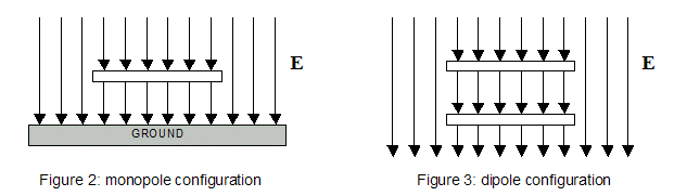
Figure 2: a single plate is placed h meters above ground. It acts as a capacitor to ground and the plate potential referred to ground is given by V = E * h. This configuration is called monopole.
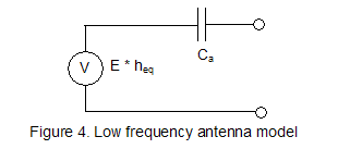
Figure 3: two plates are placed h1 meters above ground and h meters one from the other. They act as a capacitor and the differential potential between the two plates is given by V = E * h. This configuration is called dipole.
These cases can be generalized and the relationship V=E * heq can be stated even if the shape of the antenna is not a plate. In this case, the parameter heq (equivalent height) is not merely the antenna height but it is a parameter related only to the antenna physical dimensions.
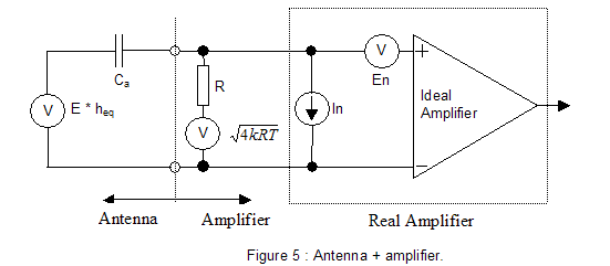
CONCLUSIONS:
The general model for an ULF or ELF antenna (monopole
or dipole configuration) irradiated by a ground wave is comprised of a
generator and a capacitor connected in series (see figure 4).
The generator has a voltage given by E * heq.
heq (antenna equivalent height) and Ca (antenna
capacitance) are both parameters related only to the geometrical configuration
and the physical dimensions of the antenna.
2. THE AMPLIFIER MODEL
Since we are considering a receiving antenna, further
considerations can be carried out by attaching an amplifier to the antenna
model.
Usually, amplifiers employed for ULF or ELF bands
exhibit very high input impedance together with a very low noise. Resistors
used for antenna loading have high value too, in the range of hundreds
of MegaOhms or GigaOhms.
Operational amplifiers based on JFET or MOSFET
technology are very popular among VLF enthusiasts and many schematics can
be found on the net and on this site too.
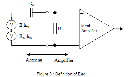
Let us consider now the schematic of a generic
ELF/ULF system shown in figure 5. It comprises the antenna, the input resistor
R and the amplifier together with their relevant noise sources.
In particular we have:
- The thermal noise of the input resistor R = sqrt 4kRT (expressed in Volt/sqrt Hz), where K is the Boltzmanns constant (1.38e-23) and T is the ambient temperature expressed in Kelvin (usually 300K)
- The thermal noise of the amplifier characterized by the parameters In and En. The former is the noise associated to the input current drawn by the amplifier (expressed in Ampere/sqrt Hz), the latter is the input referred voltage noise (expressed in Volt/sqrt Hz). Both parameters can be found on the devices datasheet where they are usually plotted versus frequency.
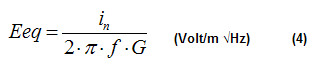
The system shown in figure 5 can be redrawn embedding all the noise sources into a single generator Eeq called input equivalent field noise. In such arrangement (see figure 6) E is the signal to receive, Eeq is the noise while the rest of the circuit is noiseless.
From the analysis of the circuit of figure 5, it can be proved that Eeq is given by:

The input signal to noise ratio (expressed in dB) at the receiver output is then:
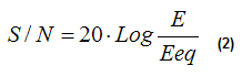
From expression (1) we can derive some important considerations:
1) The parameter Eeq is inversely proportional to
the product heq Ca (and then the signal to noise
ratio is directly proportional to heq Ca). Such product
can be considered a global performance parameter of the antenna, only dependent
on its geometrical configuration.
We will define antenna gain :
![]()
2) The parameter Eeq is inversely proportional to the frequency (f) (and then the signal to noise ratio is directly proportional to the frequency). This means that low frequencies are harder to receive than higher ones.
3) The parameter Eeq reaches its minimum value (and
then the signal to noise ratio reaches its maximum value) when R tends
to infinity. This means that it is convenient to set the resistor R at
the maximum practical value, usually in the order of few Gigaohms.
The value of Eeq when R = infinity
is given by:
4) Equation (4) suggests that In is the most important parameter when looking at an operational amplifier. It becomes the only parameter to take into consideration when R tends to infinity.
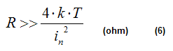
5) For practical JFET or MOSFET operational amplifiers and when R>500Mohm the contribution of En is negligible and so, the equation (1) can be simplified as follows:
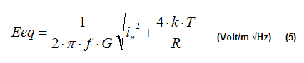
Where In is the contribution of the amplifier and the term 4*k*T/R is the contribution of the thermal noise of resistor R. Equation (4) can be used instead of (5) if:
Our goal is the reception of the background noise
at the minimum frequency with a robust signal to noise ratio. Good references
about ELF natural noise can be found on the following page:
http://www.vlf.it/naturalnoisefloor/naturalnoisefloor.htm
From plots published is this article we can roughly
set:
· At 7 Hz (first Schumanns resonance) :
100 µV/m sqrt Hz
· At 80 Hz (russian ZEVS station) : 50 µV/m
sqrt Hz
Considering +20dB of signal to noise ratio for a good reception, from (2) we can derive the required value for Eeq:
· At 7 Hz (first Shumanns resonance) : 10
µV/m sqrt Hz
· At 80 Hz (russian ZEVS station) : 5 µV/m
sqrt Hz
Next step is to calculate the required value for
the antenna gain at 7 Hz and at 80 Hz. We will perform the calculation
for two operational amplifiers (AD820 from Analog Device and LT6240 from
Linear Technology) and for R=infinity, 5 Gigaohm and 1 Gigaohm.
From equation (5) the required value for antenna
gain G is given by:
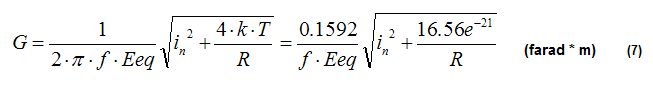
The following table summarizes the value of G calculated applying equation (7):
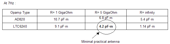
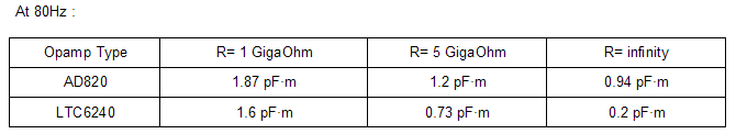
Since R=infinity is not possible (it is only a theoretical limit), the best practical choice is LTC6240 with 5GigaOhm load.
3. GAIN FACTOR EVALUATION
To complete our analysis on a minimal E-field receiver
we need a method to evaluate the antenna gain defined by equation (3).
This can be done by calculation or by simulation.
Approximate formulae are available for simple geometries such as cylindrical
monopoles or dipoles:
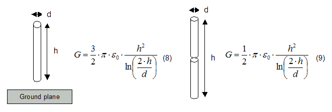
Where E 0 is the dielectric constant
of the vacuum = 8.85 pF/m
Equation (8) takes into account only the capacitance
between cylinder and infinity but not the capacitance to the ground plane
and hence it gives underestimated results.
Equation (9) is more accurate because the antenna
works without ground plane.
A very powerful method for evaluating G for any
antenna shape is by NEC2 simulator (free download available at http://www.si-list.net/swindex.html
)
Let us go back to the antenna model (see figure
4), considering the current flowing trough the antenna when short circuited.
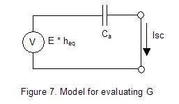
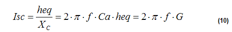
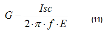
from (10) we can derive the expression for G:
To perform a NEC2 simulation we have to execute the following steps:
1) Describe the antenna geometry without voltage or current excitation points. The antenna must not have any feeding point, it must be short circuited.
2) Excite the antenna using a vertical polarized planar wave. The simulator will automatically set the field strength to 1V/m. The excitation frequency must be chosen not too low (the simulator is not intended for electrostatic analysis). A good choice is around 1/20 of the natural resonant frequency of the antenna.
3) Run the simulation and get the current at the segment corresponding to the feeding point.
4) Compute the parameter G using equation (11). E is 1V/m, f is the chosen frequency for the simulation.
EXAMPLE1 : whip monopole
GW 1 10 0 0 0 0 0 0.6 0.01
GE 1
EX 1 1 1 0 90 0 0
GN 1
FR 0 1 0 0 5 0
EN
This NEC2 code describes a 0.6meters high vertical
whip divided into 10 segments and placed above an infinite perfectly conductive
ground plane. The whip diameter is 2cm.
Excitation is accomplished by using a 5Mhz vertical
polarized wave.
Simulation gives 0.139mA of short circuit current
on segment number 1 (the one touching ground). Equation (11) gives 4.4
pFm and so this antenna can be considered minimal.
EXAMPLE2 : thick dipole
GW 1 11 0 0 3 0 0 4 0.025
GE 1
EX 1 1 1 0 90 0 0
GN 1
FR 0 1 0 0 5 0
EN
This NEC2 code describes a 1meter long vertical
dipole divided into 11 segments and placed 3 meters above an infinite perfectly
conductive ground plane. The dipole diameter is 5cm.
Simulation gives 0.146mA of short circuit current
on segment number 6 (the one at the mid point). Equation (11) gives 4.6
pFm and so this antenna can be considered minimal.
EXAMPLE3 : the cube
This example makes use of the capacitive hat
method to improve the antenna gain.
The antenna is a dipole, 30 cm of total length
and 5cm diameter. At the end of both semi-dipoles there are two plates
30x30 cm which act as capacitive hats. The whole structure is placed
3 meters above ground.
GW 106 1 -0.15 -0.15 3
-0.15 -0.05 3 1.e-3
GW 107 1 -0.15 -0.05 3
-0.15 0.05 3 1.e-3
GW 108 1 -0.15 0.05 3
-0.15 0.15 3 1.e-3
GW 111 1 -0.05 -0.15 3
-0.05 -0.05 3 1.e-3
GW 112 1 -0.05 -0.05 3
-0.05 0.05 3 1.e-3
GW 113 1 -0.05 0.05 3
-0.05 0.15 3 1.e-3
GW 116 1 0.05 -0.15 3
0.05 -0.05 3 1.e-3
GW 117 1 0.05 -0.05 3
0.05 0.05 3 1.e-3
GW 118 1 0.05 0.05 3
0.05 0.15 3 1.e-3
GW 121 1 0.15 -0.15 3
0.15 -0.05 3 1.e-3
GW 122 1 0.15 -0.05 3
0.15 0.05 3 1.e-3
GW 123 1 0.15 0.05 3
0.15 0.15 3 1.e-3
GW 136 1 -0.15 -0.15 3
-0.05 -0.15 3 1.e-3
GW 137 1 -0.05 -0.15 3
0.05 -0.15 3 1.e-3
GW 138 1 0.05 -0.15 3
0.15 -0.15 3 1.e-3
GW 141 1 -0.15 -0.05 3
-0.05 -0.05 3 1.e-3
GW 142 1 -0.05 -0.05 3
0.05 -0.05 3 1.e-3
GW 143 1 0.05 -0.05 3
0.15 -0.05 3 1.e-3
GW 146 1 -0.15 0.05 3
-0.05 0.05 3 1.e-3
GW 147 1 -0.05 0.05 3
0.05 0.05 3 1.e-3
GW 148 1 0.05 0.05 3
0.15 0.05 3 1.e-3
GW 151 1 -0.15 0.15 3
-0.05 0.15 3 1.e-3
GW 152 1 -0.05 0.15 3
0.05 0.15 3 1.e-3
GW 153 1 0.05 0.15 3
0.15 0.15 3 1.e-3
GW 206 1 -0.15 -0.15 3.4 -0.15 -0.05
3.4 1.e-3
GW 207 1 -0.15 -0.05 3.4 -0.15
0.05 3.4 1.e-3
GW 208 1 -0.15 0.05 3.4 -0.15
0.15 3.4 1.e-3
GW 211 1 -0.05 -0.15 3.4 -0.05 -0.05
3.4 1.e-3
GW 212 1 -0.05 -0.05 3.4 -0.05
0.05 3.4 1.e-3
GW 213 1 -0.05 0.05 3.4 -0.05
0.15 3.4 1.e-3
GW 216 1 0.05 -0.15 3.4
0.05 -0.05 3.4 1.e-3
GW 217 1 0.05 -0.05 3.4
0.05 0.05 3.4 1.e-3
GW 218 1 0.05 0.05 3.4
0.05 0.15 3.4 1.e-3
GW 221 1 0.15 -0.15 3.4
0.15 -0.05 3.4 1.e-3
GW 222 1 0.15 -0.05 3.4
0.15 0.05 3.4 1.e-3
GW 223 1 0.15 0.05 3.4
0.15 0.15 3.4 1.e-3
GW 236 1 -0.15 -0.15 3.4 -0.05 -0.15
3.4 1.e-3
GW 237 1 -0.05 -0.15 3.4 0.05
-0.15 3.4 1.e-3
GW 238 1 0.05 -0.15 3.4
0.15 -0.15 3.4 1.e-3
GW 241 1 -0.15 -0.05 3.4 -0.05 -0.05
3.4 1.e-3
GW 242 1 -0.05 -0.05 3.4 0.05
-0.05 3.4 1.e-3
GW 243 1 0.05 -0.05 3.4
0.15 -0.05 3.4 1.e-3
GW 246 1 -0.15 0.05 3.4 -0.05
0.05 3.4 1.e-3
GW 247 1 -0.05 0.05 3.4
0.05 0.05 3.4 1.e-3
GW 248 1 0.05 0.05 3.4
0.15 0.05 3.4 1.e-3
GW 251 1 -0.15 0.15 3.4 -0.05
0.15 3.4 1.e-3
GW 252 1 -0.05 0.15 3.4
0.05 0.15 3.4 1.e-3
GW 253 1 0.05 0.15 3.4
0.15 0.15 3.4 1.e-3
GW 1 5 0.05
0.05 3.4 0.05 0.05 3 0.025
GE 0
EX 1 1 1
0 90 0 0
GN 1
FR 0 1 0
0 5 0
EN
Simulation gives 0.151mA of short circuit current on segment number 3, wire 1. Equation (11) gives 4.8 pFm and so also this antenna can be considered minimal.
EXAMPLE4: The Romeros big Marconi
Just for comparison, let us model the antenna used
by IK1QFK for his monitoring station.
The antenna is a big T, 11 meters high with 45
meters long double hat.
GW 1 20 0 0
0 0 0 11 0.001
GW 2 10 0 -22.5 11 0
0 11 0.001
GW 3 10 0 0
11 0 22.5 11 0.001
GW 4 10 0.5 -22.5 11 0.5 0
11 0.001
GW 5 10 0.5 0
11 0.5 22.5 11 0.001
GW 6 1 0 0
11 0.5 0 11 0.001
GE 1
EX 1 1 1 0
90 0 0
GN 1
FR 0 1 0 0
1 0
EN
Simulation gives 58mA of short circuit current at
1Mhz excitation frequency on segment number 1, wire 1. Equation (11) gives
9230 pFm, about 2200 times the required minimal value.
This huge value leads to an extra signal to noise
ratio of about +67dB (!!).
4. EXPERIMENTAL CIRCUIT
Now, it is time to experiment our solution, and
see if all this mathematics will match the real world.
For this purpose I decided to try to build an antenna
as shown in Example 2 together with an amplifier based on LTC6240. For
some practical reasons some changes have been made with respect to the
original project:
- instead of using a 5cm diameter pipe I preferred to use two L-shaped profiles 5cm x 5cm (it improves the mechanical stability). The total length of the antenna is 1 meter as the original project.
- The antenna load is 4 Gohm (2x2Gohm resistors) instead of 5 Gohm because of availability problems on the market.
The experimental circuit is shown in figures 8 to 11. It is a classical schematic, similar to many we can find on the net (see, for example: http://www.vlf.it/cr/differential_ant.htm ). Here is a short description:
- stage 1 : differential amplifier based on LTC6241. R8 sets the gain. C1,C13 and C2 have been added to limit the amplifier bandwidth to about 1.5Khz. All resistors should be 1% tolerance.
- stage 2 : stage 2 : 50Hz notch filter. It is not mandatory but useful to reduce the network hum. It can be bypassed by means of switch J1. Capacitors C3,C4,C7,C8 should be 1% tolerance (possibly silver mica type).
- stage 3 : simple 2 poles, 100Hz cut-off filter. It also provides 20dB amplification.
- Stage 4 : rechargeable battery and rail splitter IC that provides the dual supply needed for the operational amplifiers.
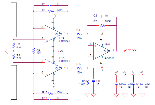
Figure 8: 1st stage : antenna and differential amplifier
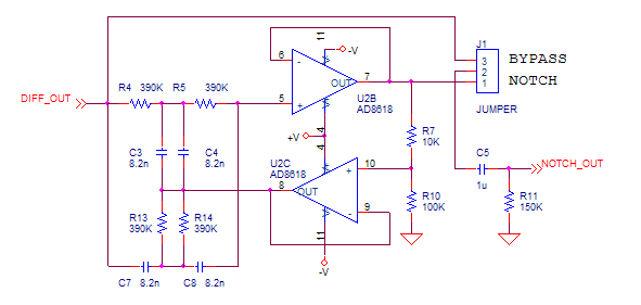
Figure 9: 2nd stage : notch
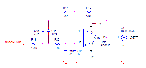
Figure 10: 3rd stage : low pass filter
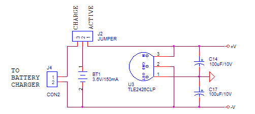
Figure 11: battery and voltage splitter
Before building the prototype, I decided to run some simulations, just to confirm the correctness of the design
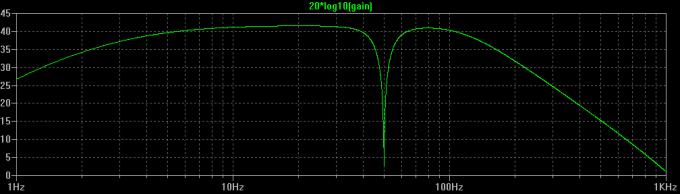
Figure 12: Simulated gain (circuit+antenna) expressed in dB.
The gain is 42dB while the 3dB lower cut-off frequency is around 3Hz.
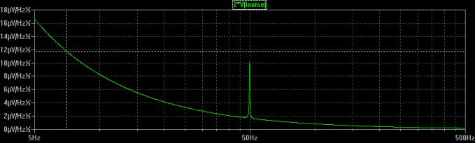
Figure 13 : Simulated input equivalent field noise (circuit+antenna) expressed in µVolt/m sqrt Hz.
The cursor set at 7Hz shows a value of 11.7 µVolt/m sqrt Hz that means a S/N ratio of 18.6dB at 7Hz (20dB was the design goal).
4. REALIZATION AND MEASUREMENTS
Finally, here is the antenna at work.
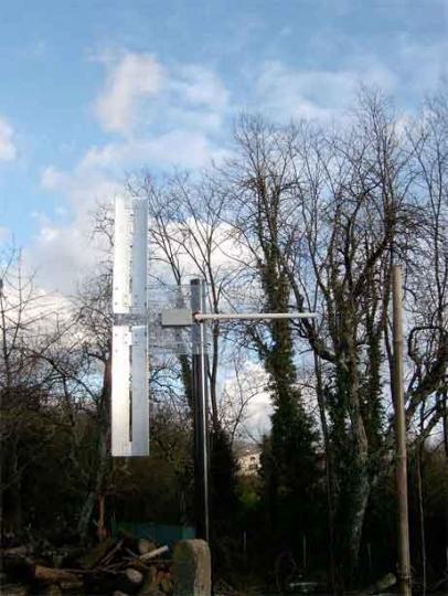
Picture 14 : the antenna at work
The first and most important measurement is the
noise margin at the 1st Schumanns resonance frequency.
As previously seen, the electronics is designed
to achieve about 19dB using the minimal antenna described in Example 2.
Since the antenna we are currently using is not strictly minimal, we expect
a margin of more than 20dB.
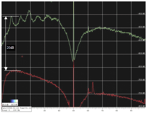
Figure 15: noise margin at 1st Schumanns resonance frequency
The spectrum above is taken on a calm, sunny day
(no wind or clouds!). FFT bandwidth was 0.127Hz, average time was about
20 minutes.
The green trace shows the background noise including
Schumanns resonances (1st to 6th), 50Hz and 60Hz hum noise while the red
one is the amplifier intrinsic noise.
The latter measurement has been made replacing
the antenna with a capacitor equivalent to the antenna capacitance (about
10pF).
The noise margin was about 20dB exactly as expected!.
This confirms our theory.
Another interesting reception is the signal coming
from ZEVS station. It is a station intended to communicating to the russian
nuclear submarine fleet.
Here below is the spectrogram taken using 10mHz
FFT bandwidth and 20 seconds scroll time. The FSK data and the 82Hz carrier
are very clear. The measured signal to noise ratio is 13.6dB.
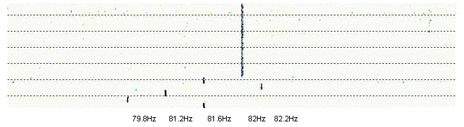
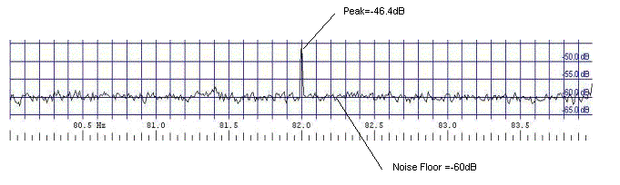
Figure 16: ZEVS reception (FSK data and S/N ratio)
The antenna is very sensitive: a severe problem
is the so called micro phonic effect , typically caused by the wind.
During the experimentation, I noticed that this
effect is especially harmful in the 0-40Hz band. Frequencies above 40Hz
seems to be not affected by microphonic effects.
Another cause of noise are moving objects near
the antenna such as tree branches (and also pets running nearby the antenna!).
This is because there is often a strong static electrical field (especially
in cloudy days) which is perturbed by moving objects.
The below spectrogram clearly shows the microphonic
effects:
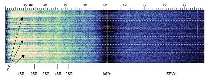
Figure 17: microphonic effects
I remember when I was a little child my grandfather
used to tell me: be quiet, we can hear the grass growing.... The antenna
is so sensitive that if placed near the ground in a windy day, it will
really detect the perturbation of the static field caused by the
grass!.
This is a good reason not to use minimal monopoles
near ground (as in Example 1).
4. ACKNOWLEDGEMENTS
IK5ZPQ Maurizio Gragnani for the mechanical construction
of the prototype.
Return to the main index of www.vlf.it