Synergistic Living with the Geomagnetic Field
John Meloy, May 2012
A recent paper in
Science
(23 March 2012: pp1466-68) described the construction
of a magnetic field cloak that rendered a
ferromagnetic object undetectable with sensors
anyplace outside the boundary of the apparatus. This,
of course, has nothing to do with observing via
magnetic fields such as we do with inductive sensors.
It is, in fact, quite the opposite. However, it
stimulated thinking; can something like this be used
to cancel the Earth's geomagnetic field and thereby
rid us of microphonic effects due to mechanical motion
of our sensor loops in that field? This
train-of-thought quickly resolved to a practical “no”
but it branched to another path. All magnetic-field
sensors based on one or more loops of a conductor and
relying on the laws of induction possess the familiar
dipole sensitivity pattern which, as we all know, has
a sensitivity zero. So, the thought path lead, “Why
not orient the sensor so that the undesired field lies
in that zero-plane?” An email dialog with this site's
creator, Renato Romero, lead to some simple
experiments and further down the mental path toward
elimination of microphonic effects. This path took us
to the desired objective and also presented a very
desirable goal achieved as a “side effect”--possible
maximization of sensitivity to natural changes in the
geomagnetic field.
The geomagnetic field is a marvelous thing. It is created largely by the flow of conductive material in the Earth's fluid outer core and changes very slowly because of the masses and processes involved. It is, for all practical purposes, a static field. It does not propagate along with an associated electric field. It is an energy storage field. If the electrical currents in the Earth that maintain it were to stop, the field would collapse and in the process transfer that stored energy to other conductors and charged particles within it. Thus the field is interactive with all electrical charges in its domain. That domain includes everything terrestrial and in the volume of space in Earth's vicinity. Thus the geomagnetic field offers us a probe with which to study everything from spaceweather to geologic dynamics.
Earth science is one of those areas interesting to laymen and scientists alike. Earthquakes both terrify and fascinate. The solar wind, never heard of a few decades ago, is now in the vocabulary of everyone. Magnetosheath, aurora, ionosphere, fault lines, and many others are words that appear not just in scientific journals, but in the public media. Scientific understanding of the independence or interaction of a wide range of once esoteric phenomena is growing quickly. The breaking and reconnection of magnetic field lines is something that was considered by no one except solar scientists a few years ago. Now we know that this happens frequently and the energy released accelerates charged particles. The aurora are a result of a rain of these particles, some from the solar wind directly, others redirected by magnetic energy release. Day-side and night-side currents in the ionosphere create telluric currents in the upper layers of the Earth's crust. Fractures and inhomogeneities in the crust cause non-uniformity in these currents and their associated magnetic fields. Sudden changes in the crust must cause changes in these near-surface currents and should be readily detectable in the local geomagnetic field. Sensors like Renato's ICS101 and others described on this site should be ideal for detection of these field disturbances.
There remains the problem of isolation of these sensors from other environmental physical effects. We do not care to detect the trembling of a heavy truck or locomotive. We do not want to “hear” rain pattering on the sheath of our sensor. We want to detect only changes in the magnetic field. The remainder of this discussion focuses on how to do that and also, hypothetically, maximize the sensitivity of our sensor to those changes. Simply stated, this hypothesis is:
Orientation of induction magnetic sensors such that the axis of the sensor is aligned with the geomagnetic field flux will minimize sensitivity to movement-induced EMF and will also maximize the sensor's sensitivity to time-varying changes in the geomagnetic field.
The first statement of this
hypothesis has been experimentally verified, although
not quantified. The second statement seems reasonable
but remains conjecture until demonstrated
experimentally. This is not an advance in science or
technology and may not even be original. It is presented
here because I have never seen it used for either
purpose and should help those using sub-Hertz-sensitive
induction sensors minimize microphonic effects. If it
also improves sensitivity to such uncharacterized
phenomena as earthquake precursors, everyone may
benefit.
The Geomagnetic Field
Wikipedia is a good and easily accessible source of information for those who wish to explore the intricacies of the geomagnetic field. This link is a good place to start: http://en.wikipedia.org/wiki/Earth%27s_magnetic_field.
For the purpose of this article we will simplify everything while staying inside the realm of reality. Consider a simple planar loop having the usual dipole sensitivity pattern within a uniform 50 μT(esla) (0.5 gauss) magnetic field. This field density is a good approximation for the total geomagnetic field in North America, Europe, Central Asia and Australia. The Wikipedia link, http://en.wikipedia.org/w/index.php?title=File:WMM2010_F_MERC.pdf&page=1, shows a global map if you wish to estimate the total field at your location. Note that this is the total field. The horizontal-field component will be smaller because of the dip or inclination of the total field. In central California the dip is about 63° measured below the horizontal (the z-axis used for geomagnetism is downward). Http://en.wikipedia.org/w/index.php?title=File:World_Magnetic_Inclination_2010.pdf&page=1 is a global inclination map. Inclination of the geomagnetic field is an important part of this discussion.
The strength and omnipresence of the Earth's field cause it to be a source of undesired effects even though it does not change very much with time. It is the time-rate-of-change of flux that induces a voltage or current in our sensor coil and physical movement of the coil can produce a time-rate-of-change that is not a signal we desire. 50 μT is huge when one considers that that magnitude is 5x10⁷ larger (154 dB, if you wish) than the average magnitude of the first Schumann resonance (about 1 pT). It does not require much physical movement of our coil to produce a flux change that will manifest as a big signal. So, what can be done when our sensor is immersed in a sea of potential microphonic signals?
During an exchange of email with Renato Romero discussing this subject, he performed a simple experiment. A hand-portable coil was repeatedly “knocked” with a wooden stick while he changed its orientation relative to the geomagnetic field vector. His results were interesting but inconclusive. He noted a “change of color” in the sound of the knocking, but the “knock” microphonic never completely disappeared. I repeated this experiment using a camera tripod for directional stability. Indeed, the “color” changed with different orientations.
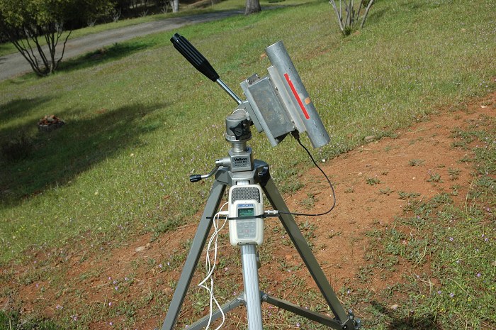
I was using a hand-held
digital recorder as a headphone amplifier and noted that
when the sensor axis was east-west and horizontal, the
“bar” deflection of the level indicator maximized when
the sensor was struck. When the sensor was oriented
north-south (magnetic, of course) the deflection was
smaller by about half. Further, when the tripod was
tilted 63° down, no deflection occurred when the sensor
was tapped with the stick. However, I could still hear
the knocking sound, but it was distinctly a much “bluer
color”.
A Myopic Viewpoint
For the sake of simplicity and ease of understanding we will restrict our view to the small volume of the geomagnetic field in the vicinity of our loop. In this volume the geomagnetic field, Be, is considered completely uniform and time invariant (dBe/dt = 0). We also assume that our loop is a simple planar surface of area Al, a valid assumption in that all coil-based sensors appear to be simple dipoles when observed from a suitable distance.
What happens when we move this loop around in this uniform static field? We know, from Faraday’s Law, that a voltage (EMF) is induced in the loop only when the flux through Al changes with time. A flux change can happen in two ways, either the field intensity changes or the loop moves, changing the enclosed flux. Since the field is invariant, movement of the coil is required to make the induced loop EMF non-zero.
If we move the loop in a fashion so that the relative angle between the uniform field and the plane of the loop does not change, the enclosed flux does not change. This means that we can wave the loop around any way we wish and not induce any microphonics—only as long as we do not change the angle between the plane of the loop and the field. Ahh haa! This says that microphonic signals in our sensor loops happen because there is some second- or higher-order motion—rotation, if you will. When we tap the sensor with a stick of wood and “hear” a microphonic signal, we have caused a rotation or some miniscule bending that has caused the flux through our device to change. This sketch illustrates the effect.
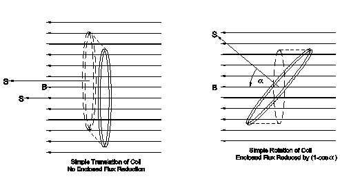
“So what?”, you ask, “That
does not solve my problem!” No, it does not solve the
problem, but it does provide a clue as to how to
minimize the microphonic problem.
The dipole field and confusion
Magnetostatics tells that our planar loop or long solenoid will, if we view it from a distance, produce the field pattern of a magnetic dipole when a current is forced through its windings. Its sensitivity to an external field, as a receiver, will have the same pattern by reciprocity. To visualize this, imagine a 3-dimensional surface of constant sensitivity. That is, the surface of induced EMF produced by a magnetic field of constant intensity, or conversely, the field intensity produced by a constant loop current. This 3-dimensional surface looks like a torus (a donut) with a “hole” diameter of zero. The torus axis, a line perpendicular to the donut and passing through its center, is also the axis, S, of the loop or solenoid. This axis is the direction of the sensitivity zeros—in a time-varying field.
This is the place where confusion is likely. We all know that if the axis of our loop is aligned with a signal source, a null occurs. This happens because the E- and associated H-field vectors are perpendicular to the wavefront (the surface of constant phase) and hence the net instantaneous flux through the coil is zero. When the plane (not the axis) of the coil passes through the signal source (or is perpendicular to the direction of arrival), the induced signal is maximized. The first idea to pass through my mind was to align the plane Al (the coil) with Be (the geomagnetic field vector). This should put the loop’s position where the net flux through it is zero. True enough, but we are not talking about an electromagnetic field, but a magnetostatic field. We are also concerned with mechanical motion that changes the angle of the coil plane with that of the field. Counter intuitively, it turns out that this orientation is exactly wrong for freedom from microphonics.
What really happens
Consider the geometry of the field and the loop. Let us forget the dipole sensitivity pattern for the moment and consider just the static flux passing through Al. If the axis of the loop (a vector perpendicular to Al), S, is aligned with the Be vector, the flux through Al is maximized, as in the sketch above. Now turn the loop so that the axis and field are no longer aligned. It is clear that the area of the loop, as seen along the field lines, is smaller and the total flux through it is less than maximum. If the angle between the sensor axis and field is α, and the flux enclosed at alignment (α = 0) is M then the flux at any angle, α, is :

In the case of a microphonic, rotation of the loop, that is, α, is a function of time and the change of flux through the loop is also a function of time. For those who have taken an elementary calculus course, you know that the derivative of a cosine function with respect to its argument is equal to the negative sine function. That is:
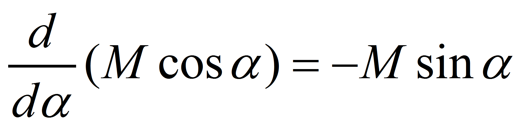
This observation provides us a clue toward minimization of angular-motion induced signals, microphonics. Note that the sine of a small angle is itself small. (In fact, a good approximation for the sine of a small angle is the angle itself, in radians. Try it with a calculator. Be certain that the units are set for radian measure.) What this means to us is that when the field and the loop axis are very nearly aligned, the flux change through the loop for small angular misalignment is itself small. Hence the induced signal in the loop due to that movement will also be small.
Note: The cosine of α is proportional to the magnitude of flux. The sine of α is the sensitivity to change of flux due to ∆α, the change in α .
Consider the case where we placed the field vector in the null of the dipole pattern, that is, with the field and the plane of the loop parallel rather than perpendicular. The angle derivative of the flux function, M(α), is still the –sine of the angle, but that angle is now π/2 and –Msin(π/2) is equal to –M. It was not at all intuitive to me that the “signal” due to coil movement when the field was in the null of the sensitivity pattern would be maximized. But that is how it turns out. This was verified by our “sensor knocking” experiment. You are are encouraged to try this simple experiment yourself.
With that observation the loop-field interaction became a bit clearer. We are not dealing with a propagating field but a static one—magnetostatic, not electromagnetic, rules are dominant here. Maxwell’s equations are still valid but the pair that describe static fields become foremost in effect. It became clear that the physics of microphonics is subtly different from signals induced by non-mechanical changes in flux density.
The sketch and the equations above imply the stated hypothesis. That is, that sensitivity to microphonics and maximization of the geomagnetic flux occur when the sensor axis and the field vector are in perfect alignment.
Determining the Direction of Be
Since we are working in a 3-dimensional world, the determination of angles requires us to use spherical geometry. Fortunately this is a well-paved road, even if we are not as familiar with it as plane geometry. In order to determine the degree of improvement that you might expect with your sensor at your location, you need to know its present axis orientation, and the magnetic declination and inclination.
You can chose any geometry you like as long as it properly represents real coordinates on the surface of a sphere. I chose to imagine my sensor located at the center of a unit-radius sphere. A plane, tangent to the Earth at the sensor's location, intersects this unit sphere and defines its equator, that is, latitude, Φ = 0. The polar axis of this sphere is a line straight up and down passing through the sensor. Since magnetic inclination (dip) is measured downward, we will call the downward pole North (ΦNP = +90°). The prime meridian (λP = 0) is defined by a vertical plane passing through the axis line and a line pointing True North from our position at the center of the sphere. Now we have a usable coordinate system.
We can easily define latitude, Φ, and longitude, λ, coordinates on our sphere and use the spherical law of cosines to find the subtended central angle between any two of them. The angle we wish to find is that between the geomagnetic field vector, Be, and the axis of our sensor, S.
Any compass direction from our point of view at the center of the sphere and looking out along the sphere-equator-intersecting plane defines a specific longitude meridian on the sphere. If we look True North (Earth-wise), the point we see is an equatorial point having coordinates ΦTN = 0 and λTN = 0. Turning our view clockwise (right) by an angle equal to the local (East) declination, we see a point with coordinates Φ = 0 and λMN = EDec (East Declination). Without turning further, look downward at an angle equal to the local dip (inclination). The point now seen has coordinates ΦB = Dip and λB = EDec. As the subscripts hint, these coordinates are those where the geomagnetic Be vector intersects our unit sphere. (If your local declination is West, you must turn left, a negative angle. If you are located south of the magnetic equator, dip or inclination will be negative. This may result in α > 90°, but since the sensor axis goes both ways, choosing the reverse projection of S resolves that. The math works in either case, only a sign change results.)
Using the orientation of your sensor axis, S, referred to True North and whatever elevation angle it may have (horizontal = 0°), find the spherical coordinates for it. The angle, α, that we seek is easily found with the spherical law-of cosines.

Recall that the geomagnetic microphonic signal induced will be proportional to:
.
Use a spreadsheet to do the work if you wish to evaluate a number of positions. But a calculator is fine for determining the improvement you can theoretically expect for one sensor at one orientation. Use either degrees or radians, but be consistent. (The approximation θ = sin(θ) mentioned earlier only works for radians and small angles.)
Example:
For my north-central California location the compass declination is 16° E and the inclination is about 63°. I have a loop whose axis is aligned with True North, so the values to plug in to the law of cosines formula become: φS = 0°, λS =0°, and φB = 63°, λB = 16°. This yields α = 65.2°, the net angle between my sensor coil axis and the geomagnetic field vector. The sine of this angle is 0.91, which means that my loop responds to 91% of the total field when it twists in the wind. This is an improvement over worst-case of less than 1 dB. If were to remount the loop by tipping it 63° toward horizontal and turning it 16° east, it would be “optimally” directed to minimize mechanical microphonics.
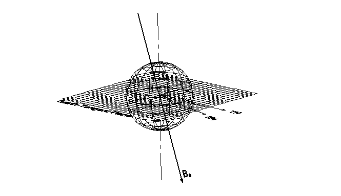
This 3-dimensional view of
the geometry used for the above calculation is shown in
this figure. The center of the sphere is the sensor
location. Magnetic North and True North are shown in the
tangent plane. The geomagnetic field, Be
is a line on the MN meridian, south of the plane at an
angle of 63° below the plane. (Apologies for the poor
legibility)
It might be instructive to calculate how much that improvement might be. Here we cannot use the derivative sine function because it is the value of sensitivity to change at exactly one point, perfect alignment, which is zero and therefore meaningless. But let us say that we are 1° from complete alignment. Then any exceedingly small change would produce a microphonic that is 0.0175M. This is an improvement of 35 dB over the worst case--and this is with a positioning error of 1°. If the alignment error can be reduced from 1° to 0.1° that microphonic is reduced another 20 dB to -55 dB from worst case. The smaller the alignment error, the greater the microphonic immunity (from worst case).
That is, as 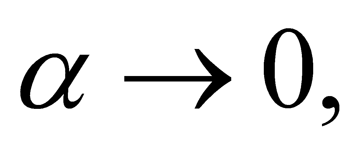
 and, in decibels,
To evaluate the exact
response of the sensor coil we need to calculate total
(normalized to 1) flux for a small range of angles
centered about 0°, find their differences, and compare
them with that same range of angles centered about what
α happens to be for the
sensor in question. This is a job for a spreadsheet.
Remember, to calculate effective total flux enclosed,
you must use the cosine of α which is proportional to the area, Al.
Keep in mind that the actual angular displacement due to
a microphonic is exceedingly small. If you wish to
equate the results to your sensor, you must keep in mind
that sensor’s frequency response. The angle α will actually be a
function of time, a vibration, if you will. We did not
state this earlier in order to minimize confusion but “α” is more accurately
stated as α(t), and
may be sinusoidal or a more complex function such as a
“knock”. The angles that you use in your spreadsheet
should be considered as the instantaneous angular
displacement from nominal.
To gain an appreciation for the small magnitude of the angles causing microphonics, let us calculate the angle that will cause a change of flux equal to the magnitude of the first Schumann resonance peak, about 1 pT. As stated earlier, the geomagnetic field in many areas of VLF monitoring activity is 50 μT. The rotation angle of any loop that changes its effective area, as seen by the geomagnetic field, by 5x10⁻⁷ depends, of course, on the loop's orientation. If the loop is optimally oriented, that angle is found by:
∆α = acos[cos(0)-5x10⁻⁷]
∆α = 0.0573° or 3.44' of arc.
A sensor oriented horizontally with its axis True North at my location has an angle, α = 65.2°, to the field vector. The rotation, ∆α, required to produce the same 1 pT change of flux is found by the ratio of the sensitivity, sin(α) at alignment and at 65.2°. This angle is extremely small.
∆α65.2 = 3.156x10⁻⁵ degrees, or 0.114 seconds of arc.
This is an extremely small angle and illustrates why microphonics are such a problem. The horizontal and TN orientation is 1810 times more sensitive to rotational microphonics than if it were oriented with the field.
Note: These calculations involving very small angles are susceptible to algorithmic and rounding errors in calculators. Computing these angles by several different methods yields different but comparable numeric outcomes. The message here is that a significant improvement is realizable. In practice, it is doubtful that accuracy of orientation better than about 1° can reliably be achieved. Even with a positioning error of 1°, the realizable reduction of microphonics is 34 dB in north-central California with a TN-oriented sensor. This is significant, particularly if it optimizes the sensitivity of time-dependent changes in geomagnetic-field intensity, i.e., geophysical signals of interest, as well.
Costs and Benefits
There are penalties to performance when a sensor is realigned from its normal position to alignment with the geomagnetic field. In most northern and southern hemisphere locations where VLF-type experimentation occurs, the dip or inclination angles are quite large. This means that the usual horizontal-plane orientation be replaced by awkwardly tilted sensors. Further, direction-finding with orthogonal loops is not amenable to this approach—only one sensor of the array could possibly benefit, its orthogonal partner is necessarily forced into the least optimal orientation. Even if your sensor system employs only one sensor, tilting it will decrease its sensitivity to signal-fields propagating along the Earth’s surface and arriving in a plane tangent to the sensor’s location. This loss of sensitivity is easy to estimate. My 63°-tilted sensor would lose 7.5 dB of its maximum sensitivity. However, the dipole null will go away, not entirely, but the azimuth “notch” may not be complete.
Considering the restrictions and potential benefits, this proposed anti-microphonic measure would best be applied to very large, very low frequency systems similar to Renato’s ICS101 solenoid. Smaller loops are generally intended for higher frequency investigations. At these frequencies, microphonics are generally not a problem and the penalties for realignment are not worth it.
Let us assume that we have aligned our ULF sensor with the geomagnetic field and are enjoying vastly reduced microphonic effects. What else can we expect? From one aspect, we have optimized our device for observation of natural causes that perturb the intensity, and to a lesser extent, the direction of the Earth’s field. We have maximized the static flux through our loop, so any time-varying change to that flux is also maximized. Remember, this idea applies to minimizing the deleterious effect due to angular motion of the sensor, not to changes in the field. Any perturbations to field intensity due to geophysical phenomena will be maximally detected. A local earthquake may shake the sensor but its response to that motion will be minimized, enabling true changes to the geomagnetic field to be distinguished. This alone may make the effort worthwhile.
This discussion has
assumed that the geomagnetic field is perfectly uniform
in the vicinity of the sensor. In the real world any
ferromagnetic object in this vicinity will concentrate
and distort the local field. This concept will still
work, but any non-uniformity of the field will degrade
the results to some degree. In addition, a nearby wire
fence moving in the wind or an automobile passing nearby
may produce time-varying distortion of the field which,
to the sensor, appears to be a valid signal. This said,
the best thing is to minimize the number and proximity
of ferromagnetic objects and to maximize the distance to
any that cannot be eliminated, moving or not.
Author's note:
This paper presents an hypothesis. Experimental verification is required before it can be regarded as anything else. The minimization of induced microphonics by field alignment is of little question. Whether detection of field fluctuations due to natural causes is maximized remains a matter of experimental verification.
I welcome critical comments or questions regarding this hypothesis, and would like to hear of any results, positive or negative, obtained from experiment.
Lastly I want to thank Renato Romero not only for his invaluable critical comments and suggestions, but for creating and maintaining an accessible web site where ideas and results can be presented for the benefit of all. Many, from academia and the professional world, visit this site and often use some of the data and ideas presented herein.
John Meloy
PO Box 2410
Mariposa, CA 95338
USA