
It has been elaborated by Daniel Labendz of the Geophysics institute of the Goettingen University in Germany, in the 1998.
Schumann Resonances reception, by magnetic component,
at less of 50,00 Euro. Can it be possible?
If yes, how can be built a minimal set-up?
And what is the cheapest way to do that?
Some answers in this article.
The starting
point: Schumann Resonances intensity
Schumann Resonances represent the arrival point
for every researcher who wants monitoring frequencies below 100 Hz, for
earthquake precursor and other applications, where the natural background
reception is required. With electric field receivers this is available
with easy and fast set-up: 2 m stylus and a high impedance preamplifier.
But the reception of the magnetic component is not that easy: very weak
values of the Resonances (as 0.5 pT) require normally the use of induction
coils. They are realised with many kg (8-10) of copper and with mumetal
core, as described in this web site and in other ones, ... with a material
cost superior to 200,00 Euro. Here we try to design and build an aerial
loop able to do that. We must face different matters: what's the minimal
set-up needed, or better how many turns? How much copper kg need? How to
amplify low noise (and cost) weak signals?
|
To be able to dimension
the reception system we need to know, first of all, the signal intensity
of the Schumann Resonances: there are many references in Internet where
the topic is developed. The results are not always homogeneous: data discrepancy
can come from season variation, geographical locations, and different detecting
system. A reasonable range exists however, and the graphic here reported
represents a good compromise.
It has been elaborated by Daniel Labendz of the Geophysics institute of the Goettingen University in Germany, in the 1998. |
A Minimal loop receiver must be sensitive enough to receive these signals, and a preamplifier must guarantee an output level able to drive a standard audio card line input.
Loop's enemy
To understand why a generic loop can't be fit to
receive these signals we need to consider who are the enemies of the weak
signal reception in the 1-100 Hz frequency range. First of all we have
a thermal noise generated by the loop resistance of the copper wire: it
works as a noise generator always turned on. Its value can easily be calculated
as follow:
Noise floor [nV/ sqrt Hz] = 4 x sqrt R [kohm] (sqrt stands for "square root")
For example: a loop with a resistance of 4 kOhm
will produce a thermal noise of: 4 x sqrt(4) = 8 nV/sqrt Hz. If the voltage
generated by the loop in the reception will be inferior to this value,
the Schumann Resonances will be buried in thermal noise, and this will
happen independently from the kind of used preamplifier. For a good loop
performance we need a loop with low resistance (and this can be obvious).
 |
A second terrible enemy is represented by the input noise voltage and by the input noise current of every amplification device: you can find this data of the operational amplifier at example in the data sheets. |
They can be represented as a noise current generator
and a noise voltage generator connected at the input of the devices ...
always turned on. Integrated circuits can have very different characteristics
and accordingly very different prices!
In the picture the input noise voltage of three
different operational amplifiers is compared. For a good loop performance
the input noise must be as low as possible, and must not overcome the signal
coming from the loop. Noise current and voltage current value can be very
different from one operational amplifier to another: best value of current
or voltage noise determines if the operational amplifier can be used with
best performance as current amplifier (as proposed follow, with low input
impedance) or as voltage amplifier (with very high input impedance).
Loop sensitivity
The aerial loops represent a more cheap solution
in comparison to the induction loop with mumetal core. But we don't know
if this solution can be adopted with success. To verify that and perform
a correct sizing of the loop (considering the loop enemy and the Schumann
Resonances intensity) we need to know the signal voltage available. Many
formulas can be used for this purpose, but the EMC (electromagnetic compatibility)
applications give simplified and practical solutions; by the Tim Williams
book (EMC for Product designers) the voltage at the loop's terminal can
be calculated as:
E[v] = (4 x 3.14 x N x A x 6.28 x F x H) / 10000000
N is the numbers of turns in the loop
A is the area of the loop in square meters
F is the frequency in Hz
H is the magnetic field in Amps/metre (or
better B[µT] x 0.796, according to the data in the first paragraph
graph)
Now we have all the mathematical elements to dimension the loop, sensitive enough to receive Schumann Resonances, over the thermal noise and the input noise of the preamplifier. We are now able to verify if an aerial loop can be sensitive enough to do that.
For example: we want to receive a signal "on air" of 5 µT at a frequency of 80 Hz. Using a squared loop of 2m shape (area 4 square meters) with 75 turns with a resistance of 35 Ohm we will find at the loop output:
E = (4 x 3.14 x 75 x 4 x 6.28 x 80 x 5 x 0.796) / 10000000 = 0.75 V
Then the loop can be connected directly to the Sound
Blaster card.
And (if the loop work below the frequency cut)
the short circuit current will be:
I = 0.75 : 80 = 9.4 mA
Some domestic
receiving loop examples
Here below some receiving loop examples. With Excel,
using the data over explained, six different "sizes" and "turns number"
loops have been simulated. Graphics show output voltage trace (violet and
brown traces) compared to the loop thermal noise (red line) and the noise
input (current and voltage both) of three different operational amplifier:
TL081 (yellow trace), OP27 (green trace) and LT1028 (white blue trace),
as indicated in the respective data sheets at the frequency value of 10
Hz. The X axes reports the frequency in Hz, the Y axes the voltage output
in Volt (indicated in exponential form). Every horizontal black grid represents
20 dB.
We start with three "casual loops", that we can realise with materials available at home: an electric wire spool (200 m of 1.5 mm insulated wire), a telephone spool (250 m of 0.6 mm pair) and a second electric wire spool (200 m, 2.5 mm) used directly as antenna.
Example n.1
 |
Loop Technical data:
Square side: 2m
Cost in Euro about 48,00 (to the hobbies supermarket)
|
An electric wire spool has been rounded around a
big wood squared shape. The loop gives signals superior to the thermal
noise (violet and brown trace represents the output voltage, based on the
levels measured by Goettingen University), but not strong enough to overcome
the noise input of TL081 and OP27. With LT1028 we have a sufficient signal
to noise ratio, but the last one is an expensive component. Besides, the
loop is big, difficult to transport, and difficult to stabilise mechanically
(an important factor that we will analyse better after here).
Example n.2
 |
Loop Technical data
Square side 0.5 m
Cost in Euro 25,00
|
A classical telephone pair spool has been rounded
on a 50 cm squared shape. The loop is little, easy to transport, easy to
stabilise mechanically. But the thermal noise cross the output voltage
trace, and any integrated circuit tested isn't sufficiently low noise to
detect the Schumann Resonances clearly.
Example n.3
 |
Loop Technical data
Circular diameter 0.3 m
Cost in Euro 130,00 (to the hobbies supermarket)
|
A classical question: can an electric wire spool be used directly as antenna? It doesn't represent a cheap solution but is already ready "as is"! I found in a supermarket a big electric copper wire spool, 30 cm diameter and 200 m length; unfortunately the graph condemns this tentative: although the received signal is over the thermal noise of the loop, the impedance is so low that any integrated circuit is able to amplify that. With this "antenna" is impossible to receive Schumann Resonances.
Some custom
project
We have seen that realising loop to receive Schumann
Resonances is not so easy and obvious. Let's go then to project some minimal
custom loops, able to receive the signal with the use of a commercial integrated
amplifier. They are realised with enamelled copper wire. The diameter chosen
corresponds to the commercial availability.
Example n.1
 |
Loop Technical data
Square side 1 m
Cost in Euro 40,00 (calculated on the basis of the
European cost of the spool enamelled copper wire, normally of 0.5 kg each
one)
|
A good compromise between cost, dimensions, sensitivity
and weight. Using an OP27 as current amplifier the Schumann Resonances
signal overcome loop thermal noise and IC input noise both. We can't use
the classical cheap operational amplifier as µ A741 or TL081,
but the OP27 is available at low cost too (about 4,00 Euro).
Example n.2
 |
Loop Technical data
Square side: 2m
Cost in Euro: 20,00 (calculated on the basis of
the European cost of the spool enamelled copper wire)
|
A more economical solution with performance similar
to the example n.3. We can use here OP27 or LT1028 both. But the dimensions
make difficult the mechanical stabilisation: for a correct reception of
Schumann Resonances the loop must be immovable, also with both wind and
rain.
Example n.3
 |
Loop Technical data
Square side 75 cm
Cost in Euro 100,00 (calculated on the basis of
the European cost of the spool enamelled copper wire)
|
Here is presented a reduced version of the 1m loop
of the example n.3. To obtain similar results we need to double the copper
weight, and consequently the cost. Where a 1 m loop represents a too big
encumbrance it can be a compromise (not very cheap).
Example n.4
 |
Loop Technical data
Square side: 50 cm
Cost in Euro 160,00 (calculated on the basis of
the European cost of the spool enamelled copper wire)
|
To realiza a little loop (50 cm squared), we need
more turns and to contain the thermal noise we need best wire section:
the copper weight grow and the cost become very high, even if the project
works.
Mechanical loop
realisation
We have chosen to realise the example number 1
(of the custom solution) as best compromise between cost and dimension.
We need to verify whether the loop really works: we don't must forget that
all the project over presented are only computer computation with an Excel
file!
 |
 |
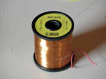
The loop has been realised using two spools of enamelled
copper wire, available in the electronic component store. Each spool weights
is 0.5 kg, wire diameter 0.2 mm, total length about 1600 m (!), and electrical
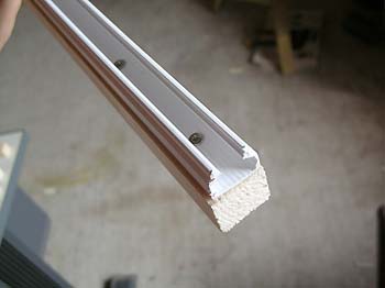
resistance 890 ohm. Four wood stakes has been assembled as a square shape,
but before a plastic guide (the one used for external electric fittings)
has been fixed to the wood with bronze screws (not magnetic), to form a
guide on the external side of the loop.
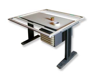 |
Another difficult comes
from the coils realisation: how to wind 3 km of thin and delicate copper
wire, maintaining a constant mechanical tension and obtaining a regular
and perfect loop?
I've used the "table technique": the squared shape has been fixed to the table surface, And I've walked around it, guiding the copper wire manually in the guide ... for some hours. It is opportune to wear before gymnastic shoes! |
There are some obvious considerations we repeat (...you never know, for novice and not only):
The low noise
preamplifier
The preamplifier is easy to build and doesn't represents
any typical difficult normally present in RF realisations. Frequency range
is so low that we need only to take care at the connections and following
the scheme.
The operation amplifier works in current, and put the loop connection in a virtual short circuit. The current value is limited by the loop resistance, and the gain comes from the ratio between 1 MOhm resistance and the loop impedance (Gain = 1000000/1800 = 555, or 55 dB). With this gain value we can connect the output directly to the Sound Blaster line input, without needed others devices. Our loop work in the range 1-100 Hz below the frequency cut, then it doesn't work in reactive zone but in resistance zone: then we can consider it as a voltage generator with a 1800 Ohm series resistance.
The VK200 is a classical RF block of some µH, to prevent cross modulation by LF and long wave signals on the integrated circuit. The 2200 µF electrolytic capacitor in input couples the loop with the amplifier, cutting the DC current: I've done different tests about, finding that cutting the DC many troubles connected with drifting and temperature changing disappear; the device results more stable. Same functions for the others two 2000 µF capacitors.

The 4.7 nF capacitor works as low pass filter: the value hasn't been chosed for flatting the frequency response, but with the purpose to obtain a reduced dynamic range in frequency spectrum. Using these values the received spectrum of the Schumann Resonances and the range up to 100 Hz appear almost flat: this helps the spectrograms reading, underlining immediately the presence of anomalous signals different from natural background noise.
Due to the very weak signals going out of the loop the suggestion is to put the preamplifier directly on the loop. The output then can be connected to the remote PC from the preamplifier with a long coaxial cable. I also tested a twisted pair telephone cable for a distance of 70 m, with no evident differences respect the coaxial solution.
The check
The loop is ready and the preamplifier too: now
is necessary to try if the project really works! We must find a quiet place:
we can't use the minimal loop in the house (and this for obvious reasons!).
An acceptable hum noise level can be found at 50 m from electric lines;
at least in my home, in the middle of the country.
 |
I've placed the loop
just outside of the garden, in the fences where my geese spend their happy
days.
This is only a temporary installation, to test if the loop works: due to the high sensitivity of the loop it must be maintained totally fixed, to avoid the microphone effect. Wind on the structure (also only a very light breeze)
or rain on it causes mechanical vibration, detected from the loop as strong
signals. For a correct work it must be buried, or covered by a protection
structure, wood or nylon.
|
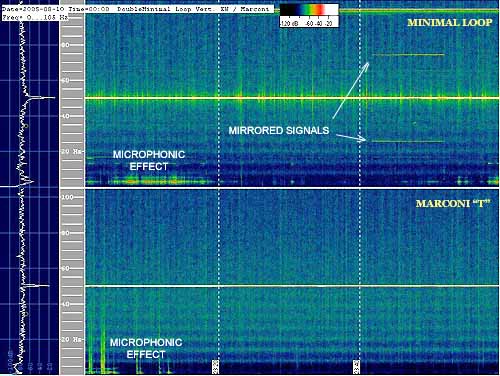
Here below the Spectrogram of 1 hour reception. The high part shows the signal received by the easyloop. Schumann Resonances are clear and evident. We can also see some mirrored tones, coming from electric lines, and microphone effect at the beginning and the end of the Spectrogram, below 10 Hz. Spectrogram below represents the same time recording of the electric component, realised with a Marconi antenna 11 m high with a double 45 m top hat: mechanical vibration causes microphone effect also here.
Conclusions
An aerial loop can be easily build to replace inductor
antenna for Schumann Resonances reception and monitoring, at a very low
price; but we need a quiet place where to place the loop, at least 50 m
far from electric lines. We must to maintain the loop perfectly locked,
to avoid microphone effect caused by mechanical movements: for this second
reason suggested dimensions are for loop of 1 meter or some less. We also
can build more small loops, but necessary copper quantity grows pushing
the price too high for a home realisation. We can build big loop too, but
they become impossible to stabilise mechanically. The
use of different operational amplifier make the difference from a Schumann
resonance active antenna and a noise generator: we can't think of the use
of µA 741 or TL081, because they are too noisy. Best compromise between
price and characteristics comes from OP27.
We can't place the receiving loop near metallic
fences or other iron structures: their mechanical vibrations deform and
modulate the earth magnetic field, producing the same microphone effects
described before.
Oh, I was almost forgetting the question at the beginning of this article: "Schumann Resonances reception, by magnetic component, at less of 50,00 Euro. Is it possible?" The answer is: "Yes, It is!"
Many thanks
to:
Marco Bruno for technical
support and measurement instruments; Wolfgang Buscher and Jader Monari
for technical revise. Andrea
Bertocchi, for English text revise.