Doing RDF (radio direction finding), one of the most delicate parts of the system is, for sure, the moving antenna. It's well known that loop or ferrite antennas can be a nuisance when operated in houses because they are too close to noise sources like computers, televisions and neon tubes. Positioning them outside the house poses some problems, in particular the installation of a rotor and the guidance of the cables to the station.
At this moment 50% of the passionate already gave up. In fact below 10 KHz, that is in the field of radio signals of natural origin, RDF is not used by anybody.
In this article we'll see how to conduct RDF using two fixed orthogonal loop antennas in combination with Cool-Edit: just a few seconds of signal recording is sufficient to find the bearing of a signal as precise as by a mechanic system.

LOOP MECHANIC DESCRIPTION
This article concerns the audio band;  the antennas have been designed  to satisfy this requirement.
 

Easyloop antennas are first choice here: it's easy to build them and they are not expensive but their performance is excellent. First of all you have to make the two orthogonal loops with  90° squared. The two loops are electrically isolated from each other and really represent two independent antennas: each one is connected with its own preamplifier from which the signals are sendt to the inputs of a two channel sound Blaster card.  So, mechanically there is no problem: shields can be in common and built for both loops in the same way. Attention: the shields must not make a closed loop, so they have to leave a gap at the top of each loop. We won't enter into technical details: everyone can proceed according his patience and ability.

The shape is not that important: round or square according to the support you use: the only required arrangement is that the planes must be at 90° to each other.
Later we'll see that the system has  a self correction device anyway, because the bearings of some RTTY stations are known. The less errors you introduce the more the measurement can be precise.
Two basic designs are recommended here. The first one is a circular loop having 40 turns of 75 cm cross section and 0.6 mm diameter wire, the second one a square loop of 66 cm side length with the same number of turns using the same wire.
Mechanically nothing is moving, so you just have to put the loop as far away as possible from electric lines, neon tubes, televisions and computers. Also avoid iron masses near the loop sides: their presence distorts radiation lobes thus altering the degrees reading.
 

DESCRIPTION OF PREAMPLIFIER CIRCUITS
Again OP27 and in fact two Easyloop preamplifiers: one for each loop. Two identical preamplifiers for two identical loops. The only difference is the orientation: the loops form an angle of 90° to each other.
We do not waist time for descriptions, because it is the same theory as described in the Easyloop article.
In order to avoid any confusion, the whole arrangement is shown here:

FIXED LOOP RDF THEORY

The loop reception lobe is bicardioid: this means a signal entering the front of the plane of the loop shows the same signal strength as a signal coming from the back - pretended both transmitters generate the same power and are equally spaced. This case is called a maximum. The loop also has a dark zone, called minimum or null at 90° to the left and right of the maximum.
I think the pattern of a figure eight polar diagram is familiar to everyone. The amplitude and phase of the current induced will depend upon the relationship between the incoming signal and the plane of the loop. This relationship follows a non linear function, the sine law for any angular position.
In other words, when the signal comes from 45°, that is between the maximal and the null position, we are not at 50% of the signal but at 70% (sin 45°=0,7).

While rotating, a single loop turning round to look for a signal encounters signals of different intensity and phase according its orientation.

The signals coming from two orthogonal fixed loops deliver informations about the phase and intensity of every single signal coming from any direction without the need of rotation, only applying the right phase and the module correction factor.
 

In other words this means that with the combination of two orthogonal loops it's possible to obtain the effect of a single loop oriented in the desired direction we need. The picture shows that an angle of, say, 45° (between north and west) can be simulated by the vectorial addition of the signals coming from the two orthogonal loops, by reducing their intensity to 70% of their maximum value, corresponding to sin 45°=0.7. The practical result is comparable to one mechanically obtained by turning around the single loop in the given direction.

Now, if this rotation by software is done according to time, then in a given time gap all possible combinations of signal strength and phase are examined and we obtain a result that contains information on signals emanating from all directions.
 

In technical terms: if we make a loop turn round 180° in 18 sec, we can obtain a spectrogram with several nulls, where time units of 100 ms correspond to angles of 1°. And of course, all of this can be realized via software. To be sure that a Null doesn't fell on the boundary of the spectrogram, an overlap of 20° has been chosen before and after the 180° margin..

Such, our creation will simulate a rotation of 220°, that is, more or less, 110° starting from the central point.

In the following table you have a list of the different amounts of the envelope which are especially needed for the module calculation length. In fact we have a sine function for one loop and a cosine for the other one.

APPLICATION WITH COOL-EDIT
After we had a look at the generic procedure theory, we can now see how it's technically possible to realize what so said. The procedure consists on four steps and provides for the realization of an audio file which contains the same information that were obtained by regular 180° rotation of a broad band loop needed for making RDF. These steps are applicated using any version of Cool Edit (sound editing software from Syntrillium, look at http://www.syntrillium.com).

A - Acquiring of 220 stereo orthogonal time units
Record the signal coming from the two orthogonal loops in a stereo .wav file, acquiring 220 time units (22 sec or 2.2 sec) and then make the angle of rotation in degrees correspond to the number of time units. If the signal is short as, for instance, a 1 sec whistler, precede with "copy/paste" creating duplicates until you have the given time span. For this procedure you can use whatever application to record wave files, but the use of Cool-edit makes things easier, since we will use it also for the following operations.

B - Envelope application
Apply the calculated envelopes to the related recorded channels. There are two ways to attain this:

Firstly you can select the channels separately one after another to apply the two attenuation functions. The envelopes can by created by selecting Transform/Amplitude/Envelope from the menu bar and editing the curves according to the table above.
  If you do not wish to create the envelope curve manually, you can use a preset function by copying the cool.ini  file in the windows directory (this file was tested with cool-edit 96. If you want to keep your own previously made definitions you can also add the lines for E-W Loop and N-S Loop to the [Envelope] section in your cool.ini file.) Thus we'll get the signal developments of a 220° rotation.

Alternatively you can perform a multiplcation of the stereo wave file with another one containing the required amplitude information. Select Edit/Mix Paste... from the menu bar and choose Modulate/From File. That file must then contain a slow sine/cosine wave of the corresponding envelope curves.
 :

This curve is simply a 220° section of one single cycle. It can be generated with cool edit once for unlimited later use. For your convenience there are two sample files for modulation ready for download: Envelope.zip (500kB). The sample rate is 44 kHz for the file of 2.2 seconds and 6 kHz for the file of 22 seconds, but it can be converted to whatever is needed.

C - Phase inversion

Once finished the preceding operation you'll have a wave file with an envelope similar to the one shown in the picture. Now you have to execute a 180° phase rotation to the signal parts which are named INVERT in the diagram: to do this just select one by one the three part to phase invert and proceed with the menu bar with Trasform/Invert. If you have chosen to use the prepared envelope wave file, this step has already been done!

D - Sample type conversion and mixing

We have so far done the envelope and the two phases of the two loops, by simulating a 220° rotation. Now we have to add the vector channel signals in order to finally obtain a resulting mono file that contains a wave simulating the loop rotation. The sample rate must be the same of the two origin channels if you wish to maintain the possibility of doing RDF on the whole monitored band. Once done save in a .wavfile.

THE SPECTROGRAM INTERPRETATION

Once obtained our final wave file we have now to decode it. In the spectrogram here shown you can see that for every single frequency a null corresponds to a given time unit, which, as  proved before, itself corresponds to the direction of the incoming signal.
Watching the spectrogram, by using the pointer it's possible to find out the frequency and the direction of a null by reading the time.
On one side of the image there is a graduated scale which shows the correspondence between time indicated by the spectrogram pointer and the direction of the incoming signals represented by a Null.
 

In the picture different signals are labelled by a yellow letter and nulls with a green one respectively; in the following table we have the spectrogram data, analyzed and interpreted.
 

LETTER	FREQ. (kHz)	Time read (s)	CALL	NAT.	Site TX	Real Direct.	Measured
A	20.9	16.1	HWU	FRA	46N37-01E05	117°	141°
B	19.8	11.0	NWC	AUS	21S47-114E09	95°	90°
C	19.6	17.0	GBZ	GB	52N43-03W04	143°	160°
D	18.3	13.4	HWU	FRA	46N37-01E05	115°	114°
E	16.4	27.0	JXN	NOR	66N25-13E54	8°	7°
F	16.0	15.8	GBR	GB	52N22-01W11	145°	138°
G	15.6	-	-	Local TV Osc.	-	-	-

In the example the development of a single recording of 22 sec is shown. If the signal in question is short, for instance 1 sec,  well have to duplicate the missing parts to obtain the required time span.  So, the same signal will be repeated several times, but the program will add, step by step, different amounts of phase resulting in the same values as obtained by a single recording.

In the example shown here the antenna was aligned correctly to the geographic orientation NS; despite this, some signals do have  mistakes concerning the direction reading , and the reason is very simple: the spectrogram was obtained with the receiving loop installed in the house, two meters away from the PC (monitor was switched off during recording). The iron armature of my house distorts the field lines and hence the lobes of loops by introducing a mistake in the measurement. Despite this we can observe that maximum mistakes do not exceed 24°.
 

ALIGNMENT OF THE RECEIVING ANTENNA

Since the provenance of some RTTY signals is known we can now do some corrections if the antenna is not correctly oriented: if the reading is some degrees apart from the real data you just have to move the antenna in the opposite direction by the same amount of degrees in order to correct for the mistake.
Sometimes signals come in phased 90° from their real direction; in this case you just have to invert one of the loops to solve the problem.
 

SOME TECHNICAL WARNINGS

The system described here is able to do even very precise measurements of the direction the signals originate from; on the whole audio band covered by the Sound Blaster card. The precision of this measurement is given by two things:

A)The two loops must be at 90° to each other. The loop orientation is not than important because the mistake of orientation can be corrected by applying a fix correction factor, easily obtained by the null of a known station. But if the angle of 90° between the two loops is not correct, it results in an orientation mistake because it cancels the trigonometric relationship of the whole system.

B) The signals of the two loops must travel from the antenna  to the station on  two different coaxial cables. You can even use twisted but shielded headphone cable (stereo) pretended that each conductor has its own shield; if not capacitive coupling between the two hot poles will produce a common signal, which moves away all nulls collecting them in a tight area of the spectrogram.

C) The receiving antenna must not encounter a magnetic mass in 1 meter distance and must not be located inside armature building. In some trials done on a balcony, to solve the problem I just had to move the loop upwards, about 70cm above the iron handrail where it had been fixed to before.

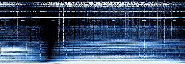
In the spectrogram shown in the picture, gotten with the theory  above written;  its possible, to observe that even hum noise has its nulls, sometimes different from frequency to frequency.

CONCLUSION
The use of a such popular device as Cool edit, and the use of cheap devices, makes this technique very interesting.  If you have wondered which direction tweaks or whistlers arrive from, you can find out for yourself now.
But a more serious question concerns the radioseismic research: with an audio acquisition system (pc and soundblaster) recording permanently but taking samples of seconds only, it's even possible to do RDF a few hours or days  later. The low cost of this technique could lead to the birth of a net, which, working on standard parameters, could be able to find the direction of suspected signals.

MANY THANKS TO:
Manfred Kerckhoff and Trond Jacobsen for the "RDF project" data.
Andrea Bertocchi and Manfred Kerckhoff for English translate.
Peter Schmalkoke and Marco Bruno for technical revise.
Steve Fazio of Syntrillium Software Corp., for authorization to use Cooledit for scientific purposes.

Return to the main index