Given the wave lengths at stake and the extreme weakness of the magnetic field to pick up, in the range of
 |
one
picotesla for the first Schumann Resonance
(SR)(3),
to compensate for the poor air permeability
the loop size must be important (about one
square meter or more) as well as the number of
enamelled cooper wire turns.
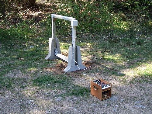
As Renato Romero remarks with salutary insistence, the microphonic effect is a major obstacle to weak signal visibility. Hence, it's absolutely necessary to limit vibration transmissions to the loop as well as possible. The first
originality of the system described in these
pages consists in the use of a heavy concrete
frame to constitute the loop frame.
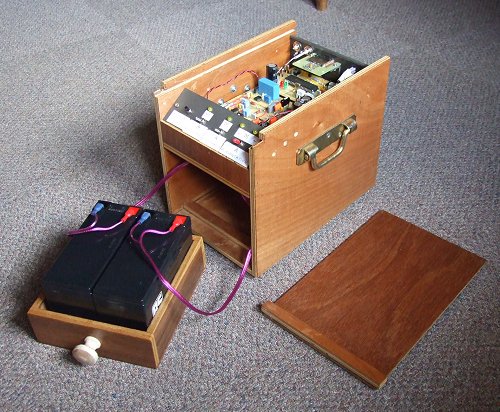
The
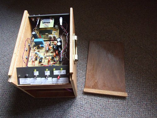
second originality lies in an embedded
recorder which allows the system to be used
far away from 50 Hz power lines and suppresses
the presence of a PC, which, as we know, also
generates electromagnetic pollution (EMP).
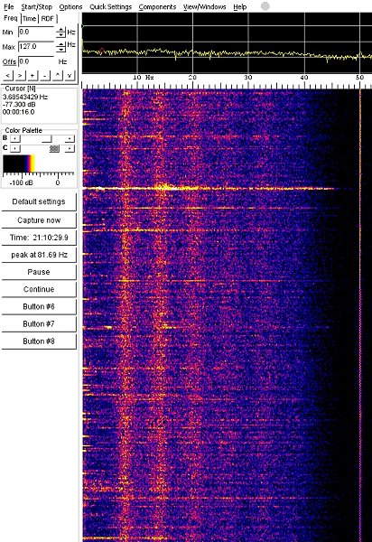
As we
shall see, the obtained results seem good, the
microphonic effect is practically absent and
the first SR very legible as we can see in the
waterfall beside.
|
|
|
 |
|
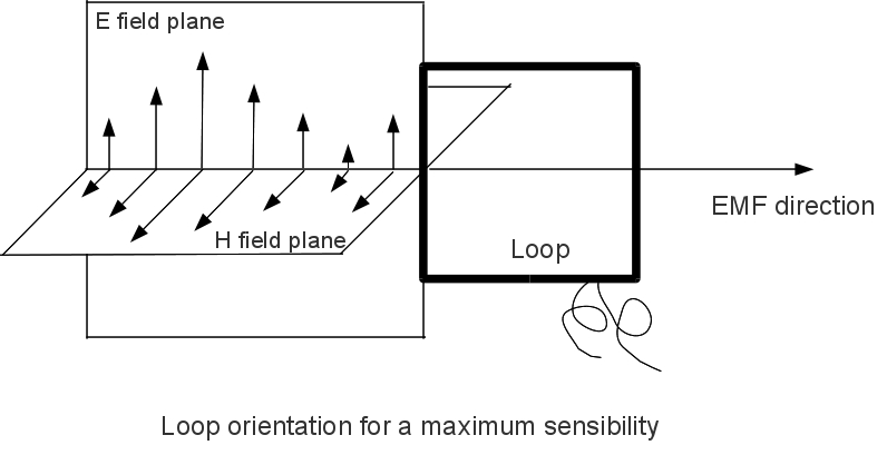
To obtain
a maximal flux, and thus a maximal induced
voltage, the magnetic field must be orthogonal
to the loop plane. Therefore to pick up a
plane polarized EMF, the loop must be in the
electric field plane.
So, for
example, to pick up a E-W directed wave (and
thus, where the magnetic field is N-S
directed), the plane must be in a N-S vertical
plane
|
But in real practice, we do
not know the nature of the numerous EM waves where we
pick up the magnetic component : some may be plane
polarized, other circular polarized, elliptic polarized,
or … not polarized. Even if we consider only plane
polarized waves, the polarization plane (which is the E
field plane) may be vertical, horizontal, or …
inclined.
 |
|
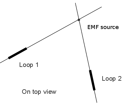
So that,
it's impossible with just one loop only to
determine the EMF direction. With two distant
loops, if we are certain to be in the presence
of a vertical polarized wave, it's possible to
determine the source position (if it's single
and defined !) orienting each loop so that the
picked up signal be maximal : it's at the two
loop planes intersecting.
Even in
the hypothetic case of a transmitter with a
corded antenna, the loop location with regard
to the transmitting antenna must be taken into
account. Indeed, the classical EMF model
described above is only avalaible at a certain
distance of the transmitter.
|
Near the transmitter, the fields E and H are neither in phase, nor orthogonal, so that the H field direction does not allow us to know the wave propagation direction. More precisely, the space surrounding a transmitting antenna is divided into three zones :
- 1°/ The reactive zone
(or near-field) in which the E and H fields are
dephased of
 ; then, the complex Poynting vector
  (and power) is purely imaginary.
 - 2°/ An intermediary zone (or Fresnel Zone) where the Poynting vector has a non-zero imaginary component.
- 3°/ The Fraunhofer zone (or far-field zone) in which the Poynting vector is purely real, E and H in phase and orthogonal. It's the standard situation which corresponds to the classical EMF model and Poynting vector gives the wave propagation direction.
However It would be useful to hold studies then the antenna size is small or very small with regard to the lengthwave, because all picked up ELF signals are not transmitted from the ionosphere or from the earth, but from various wires or human-sized devices. Thanks to Renato without whom I would have forgotten to talk about that problem.
In reality, this type of use holds little interest for us and we must abandon the hope to realize a transmitter finding system with one loop (or even two), principally because we do not know the picked-up wave nature and EFL sources are not ordinary transmitters with a classical antenna (the antenna may be the ionosphere).
So, we must consider the
magnetic field picked up in itself, and that is what we
will study. If we want to rebuilt it, we must use three
loops where the normals are respectively directed N-S,
E-W and upward. If the loops and signal conditioners are
identical, we will have the three components ![]() of the complex magnetic field
of the complex magnetic field ![]() picked up. Submitting these components
separately to spectral analysis, it's possible to
identify determined signals. From that, and knowing the
three magnetic field spectral densities, it could be
possible to have
picked up. Submitting these components
separately to spectral analysis, it's possible to
identify determined signals. From that, and knowing the
three magnetic field spectral densities, it could be
possible to have![]() approximately as a
vector for such a signal, and perhaps deduce some
information about its source. For more information, cf.
http://www.vlf.it/rdfatvlf/rdfatvlf.htm
. I specify that I have not done it and for the moment I
content myself, with only one loop where the normal is
N/S directed (to pick up
approximately as a
vector for such a signal, and perhaps deduce some
information about its source. For more information, cf.
http://www.vlf.it/rdfatvlf/rdfatvlf.htm
. I specify that I have not done it and for the moment I
content myself, with only one loop where the normal is
N/S directed (to pick up ![]() ) or E/W (to pick up
) or E/W (to pick up ![]() ).
).
The loop
I tried to reconcile :
1°/ Good electrical performances allowing to easily pick up the SRs.
2°/ A car transportable system, where each different part can be handled by one man (even if two are preferable !).
3°/ A perfect stability and a wind insensibility to avoid the microphonic effect as much as possible.
3°/ A reasonable cost. However, the loop is the most expensive part of the system.
I have chosen 0.4 mm enamelled wire, which is relatively thick, to obtain a low resistance in order to minimize the thermal noise due to the loop and enhance the Q quality factor. This wire is sold in 400-meter-long coils weighting 500 grams. Finding such coils at electronics suppliers' at a reasonable price is not always easy but possible(9). I've experimented that a length of at least 6000 m (i.e 7.5 kg) is necessary to obtain good results with a pre-amplifier mainly working in voltage(10). This represents 15 small coils of 400 m. It's easy to join these lengths end to end because the varnish is destroyed by the solder heat. However It is necessary to lightly sandpaper each extremity before twisting them together and wait a few seconds for the varnish to burn, which is visible by the emission of a pungent smoke ; a 50 W minimum soldering iron with a flat tip is necessary to bring and maintain a sufficient quantity of heat. To isolate the junction, I used a tiny piece of electrical adhesive tape but it's possible to use a special varnish.
For evident reasons, any presence of iron or magnetic metal is prohibited, that's why, in particular, the concrete is not reinforced. We subsequently can see how to palliate this difficulty. This frame, which is a main part must be made with special care : the mould must at once be very precise, solid (to be able to resist any chocks and vibrations without deformation during the concrete filling) and designed with the problem of removal and shrinkage in mind. Indeed, during setting, the concrete retracts and its size decreases while the wood keeps its length (in the fibre direction) therefore the inner mould tends to prevent the retraction and may cause the concrete to break, so, remove the moulder with care a few days later (about a week) after the concrete filling without warping the frame.
- 1°/ Fibre-reinforced concrete (with polypropylene or glass fibres). It's possible to make the mix oneself, but it's easier to buy it in bags (generally weighing 30 kg) ready to use. I recommend adding a small quantity of cement to the bags content to get a 400 kg/m3 cement dosage. The fibres won't replace steel but will improve cohesion and reduce shrinking.
- 2°/ Fibre glass textile glued on each frame face with epoxy resin in order to bring a certain tension resistance (which is theoretically nil without steel). The aim is not to make a bridge or some building but to have a sufficient resistance to be able to transport the frame without any risk (even though it will be prudent to avoid dropping it...)
Spread the resin with a spatula or a small roller over the concrete, place the fibre glass textile strip, then press it with the spatula or the roller chasing out the air bubbles (important and not always easy; do it again several times, as the textile has a tendency to raise itself if air remains under it) and lay a new resin coat above. It would be preferable to use fibre glass textile specially adapted to concrete reinforcement, but confronted with the practical impossibility of finding any in small quantities, I used solid fibre glass wallpaper. I staggered this operation on several days. The weight of the frame without the coil is about 32 kg.

Also in fibre-reinforced concrete, they are 14 cm thick and each of them weighs about 30 kg. There is no need to cover them with fibre glass textile. A layer of rubber is stuck to the bottom to receive the frame (which has also a rubber strip in the bottom). For recordings, they lie on the ground coated with a levelled sand bed. As the frame is a somewhat thick than the supports fences, I used wood wedges to block the frame.
The loop coil itself
Electrical characteristics
The pure
resistance
of the loop, measured at 20 °C is about of 870
Ohms.
Inductance
and distributed capacity.
For lack of an inductance bridge, I calculated it
by determining the resonance point when 2 different
capacitors are added in parallel on the coil and by
writing the Thompson formula ![]() in these 2 cases. I determined the
resonance point with a good quality RMS voltmeter(13). In
order to obtain a relatively sharp maximum voltage at
the loop terminals, I added big unpolarized capacitors
(1uF and 10 uF), knowing that the distributed capacity –
probably some nF - being small in front of added
capacitors, the distributed capacity given by the system
resolution would be false, but we are not very
interested in this capacity. I obtained about 65.6 Hz
with a 1uF capacitor at the loop terminals, and 18.8 Hz
with a 10 uF capacitor. The corresponding system
is
in these 2 cases. I determined the
resonance point with a good quality RMS voltmeter(13). In
order to obtain a relatively sharp maximum voltage at
the loop terminals, I added big unpolarized capacitors
(1uF and 10 uF), knowing that the distributed capacity –
probably some nF - being small in front of added
capacitors, the distributed capacity given by the system
resolution would be false, but we are not very
interested in this capacity. I obtained about 65.6 Hz
with a 1uF capacitor at the loop terminals, and 18.8 Hz
with a 10 uF capacitor. The corresponding system
is ![]() . The resolution
with Maple (or a pen !) gives
. The resolution
with Maple (or a pen !) gives ![]() (and a negligible value for C with regard
to added capacitors, as expected(14))
(and a negligible value for C with regard
to added capacitors, as expected(14))
N.B. 1°/ This method is approximative for two reasons : 1°/ The modelling of a real inductor by a pure inductor and a capacitor in parallel is questionable and sometimes gives aberrant results ; 2°/ the resonance point determination is lacking in precision. For these reasons, it's prudent to remain with only two significant digits.
2°/ It's interesting to
compare this result with the one calculated with a
formula. I have not found serious formulas giving the
inductance of such a multilayer square coil (warning :
there are fanciful formulas on the web !). Only to have
a size order, I tried to apply the formula given by http://sidstation.loudet.org/antenna-theory-en.xhtml
: ![]() (e is the coil
width – here 0.03 m -, K the square side in meters and N
the turns number) valid for a single layer coil(15). I
obtained 7.3 H exactly as before, which shows that this
value is probably near to truth.
(e is the coil
width – here 0.03 m -, K the square side in meters and N
the turns number) valid for a single layer coil(15). I
obtained 7.3 H exactly as before, which shows that this
value is probably near to truth.
3°/ Now, we can try to
evaluate distributed capacity from the resonance
frequency. This one, measured as before, is about(16) 835
Hz. Hence, the distributed capacity is about![]() .
.
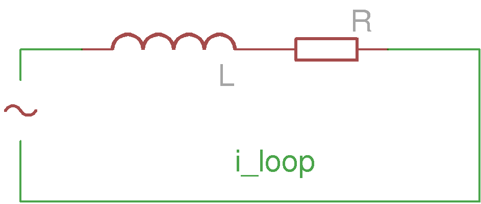
Impedance.
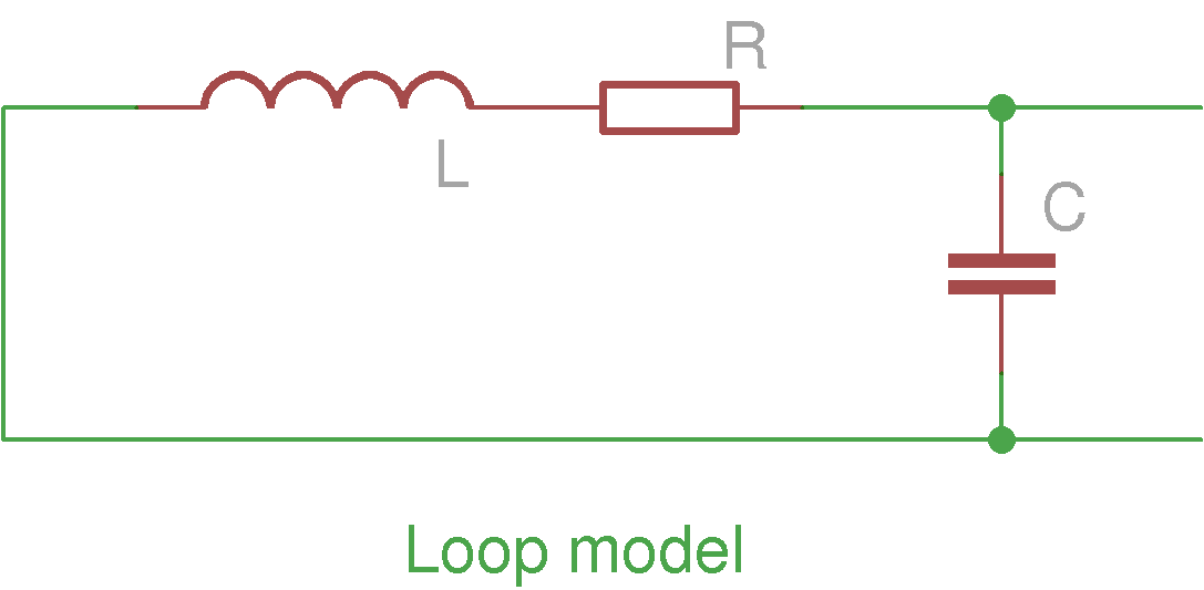
If we model the real inductor
by a capacitor C in parallel on a pure inductor L in
series with a resistor R, the impedance Z of the real
inductor is  (17); if C
is negligible, we obtain
(17); if C
is negligible, we obtain ![]() . But, is it really pertinent to neglect C
? Here is Maple worksheet, which shows that the answer
is yes in the frequency band [0, 40] if we content
ourselves with some per cent precision.
. But, is it really pertinent to neglect C
? Here is Maple worksheet, which shows that the answer
is yes in the frequency band [0, 40] if we content
ourselves with some per cent precision.

 and not
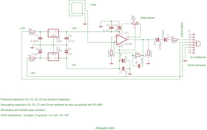

 (3)
(3)
 . This
voltage v(t) can be expanded into elementary
sinusoidal functions according to the Fourier
theory. It's generally admitted that all
frequencies are equally represented (white
noise).
. This
voltage v(t) can be expanded into elementary
sinusoidal functions according to the Fourier
theory. It's generally admitted that all
frequencies are equally represented (white
noise). 